Speaker Impedance.
A discussion on the Fun With Tubes email forum prompted the creation of this page. What is the impedance of a speaker at different frequencies? Is an eight ohm speaker really eight ohms? These questions will be answered below.
Not Frequency Response!
The curves presented below are NOT the frequency response of the speakers being tested. They are the impedance of the voice coils and associated crossover networks in speakers that have them. Note: (I would like to run frequency response curves but I can't find my calibrated microphone. I put it in a safe place that is so safe I don't know where it is.)
Instrumentation.
The instrument used to make these measurements is a SYSCOMP CGR-101.
data Presentation.
Some of you may have difficulty with the idea of presenting impedance in dB. But remember that dB is a ratio. In this case we are using the equation,
dB = 20 Log (V/I)
The network analyzer function of the CGR-101 plots a graph which is,
dB = 20 Log(V(Channel B) / V(Channel A))
So all I have to do is apply a voltage to channel A which is directly proportional to the current through the DUT (device under test). A transistor with a resistance in its emitter that is large compared to the resistance in the collector is an excellent current source.
Figure 1 Current Source to Drive Speaker.
The signal source has a low impedance and is DC coupled which eliminates the need for any biasing resistors in the base circuit. The CGR-101 inputs have no AC mode which requires an external blocking capacitor. I am sure there is at least one person shouting at their computer screen "THERE IS DC ON THE SPEAKER VOICE COIL!!!" True. But it is so small as to have no detectable effect on the results. If you own one of these instruments and you want to duplicate the results on your own speakers you may have to adjust the value of the 3.9 k ohm resistor. It's purpose is to trim the gain of the current source so it gives exactly -30 dB on the graph with an 8.00 ohm resistor connected as the DUT. The impedance is found by,
Z = 8 x 10((dB+30)/20)
For example suppose the dB reading from the graph is -25 dB.
Z = 8 x 10((-25+30)/20) = 14.23 ohms.
Reference Resistor = 8.000 ohms.
We will start by verifying the accuracy of the instrument. The resistor used has been verified to have a resistance of 8.000 ohms DC to 100 kHz and 8.00 ohms to 1 MHz
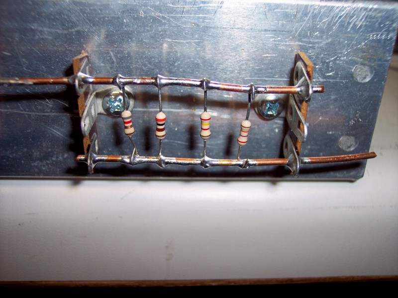
Figure 2 Photo of 8.000 ohm Reference Resistor.

Figure 3 Graph of reference resistor.
The graph deviates from -30 dB by +/- 0.13 dB. This is a resistance error of 1.51%. We will learn later that the instrument isn't really this accurate.
Eight Ohm Dummy Load Connected by its Two Foot Cable.
The measured resistance of the dummy load = 7.992 ohms through its 2 foot cable. It was measured with a DER EE LCR Meter model DE-5000. They are available all over the web, just do a Google search.

Figure 4 Photo of 8 ohm Dummy Load Resistor.

Figure 5 Graph of Dummy Load Resistor.
The graph starts out at -30.00 dB. Rises to -29.87 @ 90 to 100 kHz.
The phase = 4.8 degrees @ 75 to 100 kHz.
Koss Speaker.
These little speakers were originally part of a reverb package made by Koss, the headphone people. The idea was to place the speakers at the rear of the listening room for a pseudo quadraphonic effect. The electronics box had the reverb and two power amplifiers to drive the speakers. I was not impressed with the effect and eventually I threw the electronics away but kept the speakers. For a long time I used them as monitors for doing mixes. They are currently in disuse but I don't plan to get rid of them. They have a real good sound.
First with Short Leads.
The leads are approximately 8 inches long with alligator clips on one end and stripped ends on the other. These ends are inserted into the breadboarding socket on which the current source is assembled. Practically speaking this is about as short as the leads can be.

Figure 6 Photo of Koss Speaker.

Figure 7 Graph of Koss Speaker Connected by Short Leads.
The table below comes from the graph. While the program is live there is a cursor that gives a readout of its coordinates. While you can look at the graph I thought it would be helpful to give exact coordinates, or as exact as possible, of certain key points such as maxima and minima as well as specific frequencies along that axis. These data were entered into a spreadsheet. The column headed "Impedance (ohms)" was calculated by the formula stated above which was entered into that column. The spreadsheet was then copied and pasted into a word page and saved as a filtered HTML file. The file was then integrated into the file for this page.
|
Frequency
|
Magnitude
|
Impedance
|
Phase Angle
|
Remarks
|
|
(Hz)
|
(dB)
|
(ohms)
|
(degrees)
|
|
20
|
-30.67
|
7.41
|
10.8
|
-
|
|
50
|
-29.20
|
8.77
|
12.0
|
-
|
|
100
|
-27.20
|
11.04
|
13.2
|
-
|
|
131
|
-
|
-
|
0.0
|
Angle zero crossing.
|
|
137
|
-24.67
|
14.78
|
-6.0
|
Magnitude peak.
|
|
200
|
-28.90
|
9.08
|
-27.6
|
-
|
|
500
|
-31.33
|
6.86
|
-10.8
|
-
|
|
1 k
|
-31.60
|
6.65
|
-8.4
|
-
|
|
3.56 k
|
-
|
-
|
0.0
|
Angle zero crossing.
|
|
4.28 k
|
-33.87
|
5.12
|
-
|
Magnitude valley.
|
|
10 k
|
-32.46
|
6.03
|
25.2
|
-
|
|
20 k
|
-30.13
|
7.88
|
37.2
|
-
|
|
50 k
|
-26.06
|
12.59
|
44.4
|
-
|
|
100 k
|
-22.40
|
19.19
|
49.2
|
-
|
Koss With Five Foot Cable.
Testing speakers with 8 inch leads doesn't make much sense when it is impossible to use them that way. Oh yes, you could use monoblock amplifiers located right at the speakers or even inside the box but only the purest of the pure audio files will go to such lengths. Most of us mere mortals use leads which are a minimum of 5 feet to connect our integrated amplifiers to our speaker systems.

Figure 8 Graph of Koss Speaker Connected by Five Foot Leads.
|
Frequency
|
Magnitude
|
Impedance
|
Phase Angle
|
Ramarks
|
|
(Hz)
|
(dB)
|
(ohms)
|
(degrees)
|
|
20
|
-30.53
|
7.53
|
9.6
|
|
|
50
|
-29.20
|
8.77
|
12.0
|
|
|
100
|
-27.20
|
11.04
|
12.0
|
|
|
132
|
-
|
-
|
0.0
|
Angle zero crossing
|
|
145
|
-24.53
|
15.02
|
-
|
Impedance Peak
|
|
200
|
-28.67
|
9.32
|
-26.4
|
|
|
500
|
-31.33
|
6.86
|
-10.8
|
|
|
1 k
|
-31.47
|
6.75
|
-8.4
|
|
|
1.37 k
|
-
|
-
|
0.0
|
Angle zero crossing
|
|
4.70 k
|
-33.73
|
5.21
|
7.2
|
Impedance Valley
|
|
10 k
|
-32.46
|
6.03
|
28.2
|
|
|
20 k
|
-30.00
|
8.00
|
37.2
|
|
|
50 k
|
-25.87
|
12.87
|
45.6
|
|
|
100 k
|
-22.13
|
19.80
|
49.2
|
|
The errors between short and long leads are within the accuracy of the instrument as will be shown later. The long leads consisted of 5 feet of number 16 lamp cord, sometimes known as zip cord. This should lay to rest the claims that the speaker leads make a difference. It should but it probably won't.
Radio Shack Minimus 0.5

Figure 9 Photo of Minimus Speaker.
Radio Shack's Minimus line of products was interesting. It was a small low priced set of audio components. I used to own the amplifier and one Minimus 7 speaker. Why only one? I don't remember. I no longer can find either one so I must have given them away. A friend who was also an audio experimenter once bought 12 Minimus 0.5 speakers to play with what he called Google-aphonic sound. He tired of it rather quickly and gave me 4 of the speakers. I must have had some experiment of my own in mind but I don't remember ever carrying it out. So I have these 4 little speakers. I might as well run the impedance on them and I'll do short and long leads again to get another benchmark on the effect of leads.
Short Leads.

Figure 10 Graph of Minimus Speaker Connected by Short Leads.
|
Frequency
|
Magnitude
|
Impedance
|
Phase Angle
|
Remarks
|
|
(Hz)
|
(dB)
|
(ohms)
|
(degrees)
|
|
20
|
-30.53
|
7.53
|
1.2
|
|
|
50
|
-30.67
|
7.41
|
3.6
|
|
|
100
|
-30.53
|
7.53
|
8.4
|
|
|
200
|
-29.39
|
8.58
|
18.0
|
|
|
300
|
-24.67
|
14.78
|
0.0
|
Impedance peak
|
|
500
|
-30.40
|
7.64
|
-4.8
|
|
|
544
|
-30.53
|
7.53
|
-
|
Impedance valley
|
|
1 k
|
-30.00
|
8.00
|
7.6
|
|
|
2 k
|
-29.20
|
8.77
|
16.8
|
|
|
10 k
|
-24.67
|
14.78
|
37.2
|
|
|
20 k
|
-21.60
|
21.04
|
45.6
|
|
|
50 k
|
-17.07
|
35.45
|
49.2
|
|
|
100 k
|
-13.20
|
55.35
|
51.6
|
|

Figure 11 Graph of Minimus Speaker Connected by Long Leads.
|
Frequency
|
Magnitude
|
Impedance
|
Phase Angle
|
Remarks
|
|
(Hz)
|
(dB)
|
(ohms)
|
(degrees)
|
|
20
|
-30.80
|
7.30
|
1.2
|
|
|
50
|
-30.67
|
7.41
|
4.8
|
|
|
100
|
-30.67
|
7.41
|
7.2
|
|
|
200
|
-29.46
|
8.51
|
18.0
|
|
|
296
|
-24.80
|
14.56
|
0.0
|
Impedance peak
|
|
500
|
-30.40
|
7.64
|
-3.6
|
Impedance valley
|
|
600
|
-30.40
|
7.64
|
-
|
Impedance valley
|
|
1 k
|
-30.13
|
7.88
|
7.2
|
|
|
2 k
|
-29.20
|
8.77
|
16.8
|
|
|
10 k
|
-24.67
|
14.78
|
38.4
|
|
|
20 k
|
-21.47
|
21.36
|
48.6
|
|
|
50 k
|
-16.93
|
36.02
|
50.4
|
|
|
100 k
|
-13.07
|
56.18
|
50.4
|
|
Things seem to have changed in the wrong direction. I figure this is due to instrument warm-up rather than the effect of the leads. I think the effect of speaker leads can be largely discounted at least for the length tried so far.
The next day I tried running the curves again as close together in time as I could. The frequencies of the peak were in agreement with each other but were 291 Hz. So I guess when you pay 190 dollars for an instrument you aren't going to get HP Agilent accuracy and stability.
Due to the size of the next speakers to be tested it is no longer practical to connect them with short leads. The 5 foot length of number 16 cable will be used for all of the remaining speakers.
Sony APM-X250.

Figure 12 Photo of Sony Speaker.
I was actually forced to buy these speakers to get a Sony component TV tuner and a stereo sound adapter. Sony didn't understand the concept of component systems. They sold components as a package and wouldn't sell them parts at a time. Sony got out of the component TV business because their systems didn't sell. I wonder why? Sony was also rather stupid about the Beta VCR system. It was clearly a superior system but they refused to allow other companies to manufacture it. Meanwhile JVC, creator of the VHS system, would license anyone who asked. How different the history of TV would have been if there had been intelligent life on planet Sony. I stored the speakers for a while and eventually found a use for them.
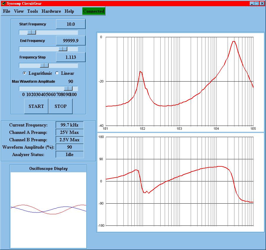
Figure 13 Graph of Sony Speaker.
|
Frequency
|
Magnitude
|
Impedance
|
Phase Angle
|
Remarks
|
|
(Hz)
|
(dB)
|
(ohms)
|
(degrees)
|
|
10
|
-31.20
|
6.97
|
9.6
|
|
|
20
|
-30.93
|
7.19
|
15.6
|
|
|
50
|
-27.87
|
10.22
|
37.2
|
|
|
84.7
|
-15.47
|
42.62
|
-
|
Impedance peak
|
|
87.9
|
-
|
-
|
0.0
|
Angle zero crossing
|
|
100
|
-17.87
|
32.33
|
-36.0
|
|
|
200
|
-29.73
|
8.25
|
-31.2
|
|
|
390
|
-31.20
|
6.97
|
-3.6
|
Impedance valley
|
|
426
|
-
|
-
|
0.0
|
Angle zero crossing
|
|
500
|
-30.80
|
7.30
|
2.4
|
|
|
1 k
|
-30.00
|
8.00
|
21.6
|
|
|
2 k
|
-27.87
|
10.22
|
38.4
|
|
|
5 k
|
-22.67
|
18.60
|
54.0
|
|
|
10 k
|
-17.47
|
33.85
|
58.8
|
|
|
20 k
|
-9.07
|
89.04
|
50.4
|
|
|
28.6 k
|
-
|
-
|
0.0
|
Angle zero crossing
|
|
29.1 k
|
-2.00
|
200.95
|
-
|
Impedance peak
|
|
50 k
|
-12.00
|
63.55
|
-76.8
|
|
|
100 k
|
-22.80
|
18.33
|
-85.2
|
|
Now I see why this speaker makes some tube amplifiers oscillate.
Radio Shack Realistic Nova 7.
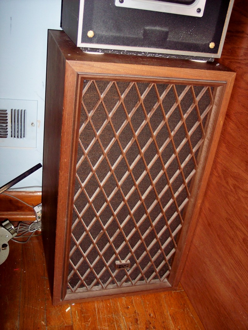
Figure 14 Photo of Nova 7 Speaker.

Figure 15 Graph of Nova 7 Speaker.
|
Frequency
|
Magnitude
|
Impedance
|
Phase Angle
|
Remarks
|
|
(Hz)
|
(dB)
|
(ohms)
|
(degrees)
|
|
10
|
-29.33
|
8.64
|
14.4
|
|
|
20
|
-28.27
|
9.76
|
26.4
|
|
|
49.7
|
-14.67
|
46.73
|
-
|
Impedance peak
|
|
50.6
|
-
|
-
|
0.0
|
Angle zero crossing
|
|
100
|
-28.53
|
9.48
|
26.4
|
|
|
139
|
-29.73
|
8.25
|
-
|
Impedance valley
|
|
180
|
-
|
-
|
0.0
|
Angle zero crossing
|
|
200
|
-28.93
|
9.05
|
3.6
|
|
|
500
|
-24.80
|
14.56
|
-
|
|
|
544
|
-
|
-
|
0.0
|
Angle zero crossing
|
|
643
|
-24.13
|
15.72
|
-
|
Impedance peak
|
|
1 k
|
-27.07
|
11.21
|
-31.2
|
|
|
2.12 k
|
-32.00
|
6.35
|
-
|
Impedance valley
|
|
2.42 k
|
-
|
-
|
0.0
|
Angle zero crossing
|
|
5 k
|
-30.13
|
7.88
|
18.0
|
|
|
10 k
|
-28.13
|
9.92
|
25.2
|
|
|
20 k
|
-26.00
|
12.68
|
31.2
|
|
|
50 k
|
-22.93
|
18.05
|
33.6
|
|
|
100 k
|
-20.40
|
24.16
|
36.0
|
|
JVC SK 500II

Figure 16 Photo of JVC Speaker.
I bought this set of speakers along with a JVC receiver to be the sound component of the AV (audio video) system that superseded the Sony components. I gave away the receiver after buying a Radio Shack AV receiver that would tune AM/FM/TV. I hung on to the speakers and they are still serving that function.

Figure 17 Graph of JVC Speaker.
|
Frequency
|
Magnitude
|
Impedance
|
Phase Angle
|
Remarks
|
|
(Hz)
|
(dB)
|
(ohms)
|
(degrees)
|
|
10
|
-29.20
|
8.77
|
25.2
|
|
|
15.3
|
-26.40
|
12.11
|
-
|
Impedance peak
|
|
18.0
|
-
|
-
|
0.0
|
Angle zero crossing
|
|
20
|
-27.33
|
10.88
|
-2.4
|
|
|
42.0
|
-29.33
|
8.64
|
-
|
Impedance valley
|
|
42.1
|
-
|
-
|
0.0
|
Angle zero crossing
|
|
50
|
-29.06
|
8.91
|
3.8
|
|
|
72.4
|
-
|
-
|
0.0
|
Angle zero crossing
|
|
75.8
|
-24.80
|
14.56
|
-
|
Impedance peak
|
|
100
|
-29.33
|
8.64
|
-27.6
|
|
|
167
|
-31.73
|
6.56
|
-
|
Impedance valley
|
|
190
|
-
|
-
|
0.0
|
Angle zero crossing
|
|
200
|
-31.47
|
6.75
|
0.6
|
|
|
500
|
-29.73
|
8.25
|
19.2
|
|
|
1 k
|
-26.27
|
12.29
|
20.4
|
|
|
1.80 k
|
-
|
-
|
0.0
|
Angle zero crossing
|
|
1.91 k
|
-23.07
|
17.77
|
-
|
Impedance peak
|
|
5 k
|
-32.40
|
6.07
|
-31.2
|
|
|
7.45 k
|
-34.40
|
4.82
|
-
|
Impedance valley
|
|
7.59 k
|
-
|
-
|
0.0
|
Angle zero crossing
|
|
10 k
|
-33.47
|
5.37
|
16.8
|
|
|
20 k
|
-29.73
|
8.25
|
37.2
|
|
|
50 k
|
-24.93
|
14.34
|
44.4
|
|
|
100 k
|
-21.33
|
21.71
|
44.4
|
|
SPL 99.

Figure 18 Photo of SPL 99 Speaker.
SPL stands for Sound Power Laboratories. I have saved the best for last. These are my primary listening speakers which are part of the best system in the house. I bought them in 1972, I think, After some careful listening. I think they were about $200 or $250 each. That was a lot of money in those days when you could buy a house for $18,000 and a new car for $3600.
The woofer is an acoustic suspension type. About 10 years ago the rim around the woofer disintegrated as old plastic is want to do and I had to replace the woofers with some from Radio Shack. The bass was almost as good but there was a small difference.

Figure 19 Graph of SPL 99 Speaker.
|
Frequency
|
Magnitude
|
Impedance
|
Phase Angle
|
Remarks
|
|
(Hz)
|
(dB)
|
(ohms)
|
(degrees)
|
|
10
|
-30.67
|
7.41
|
9.6
|
|
|
20
|
-30.40
|
7.64
|
8.4
|
|
|
50
|
-26.40
|
12.11
|
9.6
|
|
|
53.4
|
-
|
-
|
0.0
|
Angle zero crossing
|
|
54.4
|
-25.87
|
12.87
|
-
|
Impedance peak
|
|
69.4
|
-
|
-
|
-20.4
|
Angle Valley
|
|
100
|
-
|
-
|
-4.8
|
|
|
106
|
-31.33
|
6.86
|
-
|
Impedance valley
|
|
144
|
-
|
-
|
0.0
|
Angle zero crossing
|
|
200
|
-29.60
|
8.38
|
9.6
|
|
|
356
|
-27.47
|
10.71
|
0.0
|
Impedance peak
|
|
500
|
-28.53
|
9.48
|
-10.8
|
|
|
1 k
|
-31.33
|
6.86
|
-9.6
|
|
|
1.42 k
|
-
|
-
|
0.0
|
Angle zero crossing
|
|
1.50 k
|
-31.87
|
6.45
|
-
|
Impedance valley
|
|
2 k
|
-31.73
|
6.56
|
8.4
|
|
|
5 k
|
-29.73
|
8.25
|
20.4
|
|
|
10 k
|
-27.73
|
10.39
|
26.4
|
|
|
20 k
|
-25.73
|
13.08
|
27.6
|
|
|
50 k
|
-23.33
|
17.24
|
30.0
|
|
|
100 k
|
-21.07
|
22.37
|
34.8
|
|
I think you can tell by the graphs and numbers that these really are the best speakers in the house.
Conclusion.
For all of my life I have heard that the impedance of a speaker is quite variable over the audio frequency range. I didn't doubt it but I have only seen one speaker manufacturer who published impedance curves for their speakers. I think the curves were fore the Altec-Lancing Voice of the Theater. That speaker system has always been financially out of reach for me. Even that stratospheric end system had a lot of variability.
My SPL systems have an impedance variation of -25% to +50% which seems like a kindness to amplifiers. Whether tube or transistor, an amplifier would prefer to drive an impedance that is higher than it was designed for rather than lower.
Measurements on Your Speakers.
If you want to know what the impedance versis frequency of your speakers is you can buy the instrument for 190 dollars. I have given enough information to enable you to duplicate the experiment on your own. If you would like me to do it for you I will for a price. And in addition you have to pay for shipping both ways. Clearly it would be less expensive to just pay the 200 dollars and get the instrument.
This page last updated April 6, 2014.
Home>