Chapter 1 Perception and Theory of Distortion.
1.1 The Theory of Measuring THD (Total Harmonic Distortion).
1.1.1 Input Attenuator and Input Buffer. 1.2 The Theory of Measuring IMD (InterModulation Distortion).
1.1.2 The Notch Filter.
1.1.3 The Voltmeter.
1.1.4 The Output
1.1.5 Making the Measurement.
1.1.6 How all this Works Together.
1.1.7 An Alternate Method.
1.2.1 Test Signal Generator. 1.3 How We Perceive Distortion.
1.2.1.1 Low Frequency generator. 1.2.2 Input Attenuator.
1.2.1.2 High Frequency Generator.
1.2.1.3 Linear Mixer.
1.2.1.4 Output Buffer.
1.2.3 Input Buffer.
1.2.4 High pass filter.
1.2.5 Detector (Rectifier.
1.2.6 Low Pass Filter.
1.2.7 The Meter.
1.2.8 Instrument Calibration by the DC method.
1.2.9 Calibration by the Two Signal Method.
1.3.1 Harmonic Distortion. 1.4 The mathematics of distortion.
1.3.2 Intermodulation Distortion.
1.4.1 Harmonic Distortion and the Gain Polynomial./ 1.5 Conclusion.
1.4.1.1 The Gain Polynomial. 1.4.2 Intermodulation Distortion.
1.4.1.2 The Input Signal.
1.4.1.3 Amplitudes of the Harmonics.
1.4.1.4 Example.
1.4.2.1 The Gain Polynomial.
1.4.2.2 The Input Signal.
1.4.2.3 The Binomial Theorem.
Chapter 1 Perception and Theory of Distortion.
Since 1950 many ordinary audiophiles have been puzzled over why some amplifiers with good specifications just don't sound right while some others with specifications that are not as good as one might want still sound good. I don't pretend that I can set this argument to rest but perhaps I can cast a little light into the darker corners of the discussion.Back to Fun With Tubes.
Back to Fun With Transistors.
Back to Table of Contents.
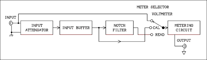
Back to Top.1.1 The Theory of Measuring THD (Total Harmonic Distortion).
This section may appear to be off topic and it probably is. It is included to make the discussion complete.The instruments which are used to measure THD (total harmonic distortion) are made up of two basic elements. 1) a sharp and deep notch filter capable of attenuating a single frequency by at least 90 dB while leaving all other frequencies unchanged in amplitude. 2) a voltmeter with a dynamic range of 90 dB and an upper frequency limit of approximately 10 times the highest frequency at which distortion is to be measured. A typical instrument also includes an input attenuator, an input buffer, and a notch filter output.
Back to Fun With Tubes.
Back to Fun With Transistors.
Back to Table of Contents.
Back to Top.1.1.1 The input attenuator and input buffer.
The input attenuator is used to adjust the input level so the instrument can be used over a wide range of input voltages. The Vernier of the attenuator is also used to adjust the instrument to read 100% for the particular input signal level.The input buffer provides a high input impedance so the instrument will not load single stage circuits that are being tested in a standalone condition.
Back to Fun With Tubes.
Back to Fun With Transistors.
Back to Table of Contents.
Back to Top.1.1.2 The Notch Filter.
A filter constructed using all passive components cannot meet the requirements as stated above. A practical filter consists of a combination of passive components and a high gain amplifier. The amplifier is arranged so as to feed the output signal back to cancel the input signal at a single frequency. Detailed circuitry is beyond the scope of this chapter.Back to Fun With Tubes.
Back to Fun With Transistors.
Back to Table of Contents.
Back to Top.1.1.3 The Voltmeter.
The voltmeter is really nothing special. Measurement companies such as Hewlett Packard, Fluke, and General Radio, have been making standalone AC voltmeters for decades. In an instrument made to measure THD the built in meter range switch has some additional labeling for ranges starting at 100% usually the 0.3 volt range and going down to 0.1% or 0.03% depending on the particular instrument.Back to Fun With Tubes.
Back to Fun With Transistors.
Back to Table of Contents.
Back to Top.1.1.4 The Output.
Every THD analyzer I have ever seen has a set of terminals labeled "Output". The signal available on these terminals is taken from the metering circuit after the meter range switch. This signal has many uses. A true RMS meter may be connected for a more accurate reading of the harmonics in case the instrument does not incorporate such a meter. Also the signal can be fed to an oscilloscope or a spectrum analyzer to examine the harmonic content without the large fundamental frequency getting in the way.Back to Fun With Tubes.
Back to Fun With Transistors.
Back to Table of Contents.
Back to Top.1.1.5 Making the Measurement.
The frequency of the notch filter is user adjustable, well it wouldn't be much use if it wasn't, and the balance of the circuit is as well. The output of a low distortion sine wave generator is fed to the input of the amplifier under test. The levels are adjusted so the amplifier is operating at the desired power level and the output signal of the amplifier is fed to the input of the THD analyzer. With the filter switched out the input attenuator is adjusted until the signal indicates 100% on the meter. Then the filter is switched in and adjusted for the lowest possible reading on the meter. Modern instruments have an automatic adjustment circuit that may be switched on after the reading has been manually reduced below about 3%. As the reading gets lower the range switch on the meter is changed and when the reading is as low as it can get the distortion is read from the meter.Back to Fun With Tubes.
Back to Fun With Transistors.
Back to Table of Contents.
Back to Top.1.1.6 How all this Works Together.
The notch filter is adjusted to the fundamental frequency of the oscillator signal and the fundamental is effectively removed from the scene. What is left are the harmonics and unless the amplifier is perfect there will be some. For best results the meter should read in true RMS (root mean square) but there are many which do not.Back to Fun With Tubes.
Back to Fun With Transistors.
Back to Table of Contents.
Back to Top.1.1.7 An Alternate Method.
Another way to do it is to use a spectrum analyzer or wave analyzer to read the voltage of the fundamental frequency plus the voltage of each harmonic. The total harmonic distortion is then found by,THD = 100% sqrt(H22 + H32 + . . . + Hn2)/H1 Where H1 is the amplitude of the fundamental frequency, H2 the amplitude of the second harmonic, H3 is the amplitude of the third harmonic, Hn is the amplitude of the nth harmonic, and sqrt denotes taking the square root of the value inside the following parentheses. This system is quite cumbersome but, for instance, there may be occasions when the design engineer wants to know the relative amplitudes of even and odd numbered harmonics. We will revisit this question in a later section of this chapter. Also taking the square root of the sum of the squares is what a true RMS voltmeter does.
Back to Fun With Tubes.
Back to Fun With Transistors.
Back to Table of Contents.
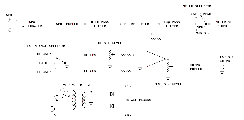
Back to Top.1.2 The Theory of Measuring IMD (InterModulation Distortion).
First we describe the test instrument. The instrument which is used to measure IMD (InterModulation Distortion) is made up of 7 parts. 1) A special test signal generator (which itself is actually made up of 4 parts LF GEN, HF GEN, the op amp, and the OUTPUT BUFFER),, 2) The input attenuator, 3) the input buffer, 4) a high pass filter, 5) a detector (rectifier circuit), 6) a low pass filter, and 7) a voltmeter with a dynamic range of 90 dB.
Back to Fun With Tubes.
Back to Fun With Transistors.
Back to Table of Contents.
Back to Top.1.2.1 Test Signal Generator.
The test signal generator consists of 4 parts. 1) a low frequency generator, 2) a high frequency generator, 3) a linear mixer, and 4) an output buffer..Back to Fun With Tubes.
Back to Fun With Transistors.
Back to Table of Contents.
Back to Top.1.2.1.1 Low Frequency generator.
In North America the low frequency generator has a frequency of 60 Hz. It may be derived directly from the 60 Hz line or it may be an oscillator which is locked to the line frequency. In either case it should be as free from distortion and noise modulation as possible. The reason for locking to the line frequency is to avoid beat frequencies which would cause the meter to slowly waver.Back to Fun With Tubes.
Back to Fun With Transistors.
Back to Table of Contents.
Back to Top.1.2.1.2 High Frequency Generator.
The high frequency generator has a frequency of 7,000 Hz. It is especially important that this signal be as free from noise modulation as possible. Any noise on this signal will be read as IM distortion by the metering circuits.Back to Fun With Tubes.
Back to Fun With Transistors.
Back to Table of Contents.
Back to Top.1.2.1.3 Linear Mixer.
A radio engineer reading this text may be confused at this point. This is not a mixer that is intended to produce sum and difference frequencies as in the mixer in a radio receiver. In fact it is designed to do just the opposite. Sum and difference frequencies, if they exist in the output of the test signal generator will be read as IM distortion by the measuring circuit. The mixer is designed to perform linear addition of the two voltages from the two generators without producing any sum and difference frequencies. It is usual for the two signals to have an amplitude ratio of 4 to 1 with the 60 Hz frequency having the largest amplitude. The output of the mixer is fed to the amplifier under test.Note: I do not know what frequencies are used for IMD measurement in the rest of the world. Perhaps someone who lives there will enlighten me.
Back to Fun With Tubes.
Back to Fun With Transistors.
Back to Table of Contents.
Back to Top.1.2.1.4 Output Buffer.
The output buffer is designed to provide a relatively low output impedance so as to drive any load that the user may present to it. In high end instruments the output impedance is likely to be 50 ohms and it may include a step attenuator to provide a wide range of output voltage.Back to Fun With Tubes.
Back to Fun With Transistors.
Back to Table of Contents.
Back to Top.1.2.2 Input Attenuator.
The output of the AUT (amplifier under test) is fed to the input of the instrument where the first section it encounters is the input attenuator. This attenuator allows a wide range of input voltages to be applied without overloading or even burning out the input buffer amplifier. For example a 200 watt amplifier will supply 40 volts across 8 ohms. While the output level of a preamplifier or mixing console may be 0.7 or 0.5 volts. An IM analyzer must be capable of operating properly under both of these extremes and all points between. The Vernier of the attenuator is adjusted to standardize the instrument to 100%.Back to Fun With Tubes.
Back to Fun With Transistors.
Back to Table of Contents.
Back to Top.1.2.3 Input Buffer.
The input buffer must provide a high input impedance to enable the instrument to be used to test individual amplifier stages which may not have a low output impedance. Field effect transistors are usually employed. The amplifier may have a voltage gain of unity or may have a higher gain.Back to Fun With Tubes.
Back to Fun With Transistors.
Back to Table of Contents.
Back to Top.1.2.4 High pass filter.
After being attenuated and buffered the signal from the AUT is fed into the high pass filter.)The purpose of this filter is to remove any detectable trace of the 60 Hz signal from the output of the AUT.Back to Fun With Tubes.
Back to Fun With Transistors.
Back to Table of Contents.
Back to Top.1.2.5 Detector (Rectifier.
The detector follows the high pass filter. The only signal left after the high pass filter is the 7,000 Hz signal plus any sidebands due to it being amplitude modulated by the 60 Hz signal. Such modulation takes place if the two signals have passed through any nonlinear elements. If nonlinearities exists within the AUT such modulation of the 7000 Hz signal will be present. The detector works exactly like the detector in an AM radio receiver and will produce an output of 60 Hz if any such modulation is present. We will learn more about this in section 1.4.Back to Fun With Tubes.
Back to Fun With Transistors.
Back to Table of Contents.
Back to Top.1.2.6 Low Pass Filter.
The low pass filter removes any measurable 7000 Hz signal leaving only the recovered 60 Hz modulation.Back to Fun With Tubes.
Back to Fun With Transistors.
Back to Table of Contents.
Back to Top.1.2.7 The Meter.
A selector switch on the instrument selects a calibration signal that defines 100% modulation of the 7000 Hz signal. The input level is set so the meter will indicate 100% and the switch is changed to read the output of the low pass filter. The meter range switch is changed until a reading can be obtained.Back to Fun With Tubes.
Back to Fun With Transistors.
Back to Table of Contents.
Back to Top.1.2.8 Instrument Calibration by the DC method.
At the output of the rectifier the output looks like, and in fact is, a full wave rectified sinewave. The negative going peaks are at ground potential. The positive going peaks are at the peak level of the "carrier", 7000 Hz signal. Thus there is a DC level at the output of the rectifier that is proportional to the level of the 7000 Hz signal. For convenience let's assume that the RMS level of the "carrier" is 1 volt. The peak level will be 1.41421 volts. The Low pass filter takes the average value of the rectified signal. That makes the DC level 0.636620 x 1.41421 V = 0.899723 volts. The low pass filter is DC coupled so this DC is passed on through while all measurable traces of the 7000 Hz signal itself are to all intents and purposes removed.The DC level at the output of the low pass filter is 0.899723 volts. Note that this so called DC level is capable of changing at a 60 Hz rate. If the "carrier" were to be 100% modulated its peak value would change from 0 to twice the static peak so the level at the output of the low pass filter would change from 0 to 1.79945 volts. Thus for 100 % modulation the peak to peak sinusoidal voltage at the output is 1.79945 volts. Converting this to RMS gives 0.63620 volts. Remembering that the unmodulated DC output is 0.899723 volts the ratio of the unmodulated DC to the RMS AC for 100% modulation is 1.41421. We shouldn't be surprised by that. So, if we want 100% to equal 1 volt RMS we should set the DC level to 1.41421 volts DC.
This sounds good in theory but the practical limitation is that the low pass filter has a slightly different gain for AC and DC. There may be some difference between different builds of the detector and filter circuit so another means must be found to calibrate the instrument.
Back to Fun With Tubes.
Back to Fun With Transistors.
Back to Table of Contents.
Back to Top.1.2.9 Calibration by the Two Signal Method.
The standard method of calibration is to produce a 7000 Hz signal that is amplitude modulated at a well-known modulation percentage. A very easy and accurate way of doing this is to turn off the 60 Hz signal from the test signal generator and insert another signal that is 60 Hz higher than the HF generator and exactly 1/10 the amplitude. This single sideband signal with carrier is treated by the detector the same as a double sideband signal with carrier that is modulated at 10%. The signal is fed to the test circuit and the calibration adjustment is set for a reading of 10% on the meter.Back to Fun With Tubes.
Back to Fun With Transistors.
Back to Table of Contents.
Back to Top.1.3 How We Perceive Distortion. Although I treat harmonic and intermodulation distortion separately in the following discussion this is unrealistic. The two are caused by nonlinearities in the amplifier and are inseparable.
Back to Fun With Tubes.
Back to Fun With Transistors.
Back to Table of Contents.
Back to Top.1.3.1 Harmonic Distortion.
Every note played by a band produces harmonics but this gets impossible to handle in an example such as this. Therefore we will use one note C4 or middle C which has a frequency of 261.63 Hz. The second harmonic is exactly an octave higher and does not add any dissonance to the music. The third harmonic is 784.88 Hz. This is only 0.89 Hz higher than G5 which reinforces the 5th note of the C chord while adding a slow vibrato to the music. The 4th harmonic is exactly 2 octaves higher than C4 and will do mo more than add a little tambour to the note. The 5th harmonic is 1308.13 which is about 10 Hz below E6 and reinforces the 3rd of the C chord. The 6th harmonic is less than 2 Hz above G6 which once again reinforces the 5th note of the scale. The 7th harmonic is 33 Hz below Bb6 which reinforces that flatted seventh chord that is used so often in country and folk music.We are up to the seventh harmonic and we have yet to create any really dissonant notes. We don't get any notes that are seriously out of tune until the 9th harmonic which is 5 Hz higher than a D7*.
* This does not mean the D7 chord which is often played as the fourth chord in the key of C, but the d in the seventh octave.
The higher the harmonic number the lower the amplitude and the truth is the high order harmonics are below the noise floor of most amplifiers and so aren't perceived by the listener. So if all this is true why does distortion sound so bad?
If we could make an amplifier that would produce only harmonic distortion and no intermodulation distortion we wouldn't have to worry about it as much as we do. Distortion is produced by nonlinearity in the amplifier. I will discuss this in the next section. Any nonlinearity will produce both harmonic and intermodulation distortion and it's the IM distortion that sounds so bad.
Back to Fun With Tubes.
Back to Fun With Transistors.
Back to Table of Contents.
Back to Top.1.3.2 Intermodulation Distortion.
Intermodulation distortion does not produce harmonics that are in basic tune with the musical scale but sums and differences that are usually out of tune. For example suppose a C major chord is being played in the 5th octave. G5 has a frequency of 783.99 Hz and E5 a frequency of 659.26 Hz. The sum is 1443.25 Hz which is between F and F# in the 6th octave. The difference is 124.73 which is a little more than a hertz above a B2. Both of these notes are quite dissonant when played along with a C major chord. This is why an amplifier with distortion sounds so unpleasant.So we conclude that IMD is much more objectionable than THD. As stated earlier the two go together like love and marriage, a horse and carriage, or any other pair you might care to name. I am not advocating abandonment of THD measurements. I think that we audio hobbyists should measure IMD alongside THD for a complete picture of the behavior of an amplifier.
Back to Fun With Tubes.
Back to Fun With Transistors.
Back to Table of Contents.
Back to Top.1.4 The Mathematics of Distortion.
Here we will treat harmonic distortion and then dig into intermodulation distortion. A single frequency test signal will be used to evaluate the gain polynomial of a real amplifier. Then a two frequency test signal will be run through the polynomial to see what other frequency components come out.Back to Fun With Tubes.
Back to Fun With Transistors.
Back to Table of Contents.
Back to Top.1.4.1 Harmonic Distortion and the Gain Polynomial./
An amplifier can be characterized by a polynomial and the coefficients found for a real amplifier if desired. While the procedure is a bit tedious it can be useful to those who want to design quality amplifiers.Back to Fun With Tubes.
Back to Fun With Transistors.
Back to Table of Contents.
Back to Top.1.4.1.1 The Gain Polynomial.
Most of us are accustomed to thinking of gain as a real number. Note: Dealing with phase shifts will only make things unnecessarily more complicated so we will not try to deal with imaginary numbers. The gain of an amplifier is not truly linear. It must be represented as follows.f(Vin) = A0 + A1Vin + A2Vin2 + A3Vin3 + . . . + AnVinn
Back to Fun With Tubes.
Back to Fun With Transistors.
Back to Table of Contents.
Back to Top.1.4.1.2 The Input Signal.
Testing for harmonic distortion requires the input signal to be a pure sinusoid. For the following analysis the input signal will be,Vin = V cos (ωt) where V is the peak value of the signal, ω is the angular frequency in radians per second, ω = 2 π f where f is the input frequency in Hz, and t is time in seconds.
Back to Fun With Tubes.
Back to Fun With Transistors.
Back to Table of Contents.
Back to Top.1.4.1.3 Amplitudes of the Harmonics.
We will substitute Vin = V cos (ωt) into the above equation and carry it out to N=4.f(Vin) = A0 + A1V cos (ωt) + A2V2 cos2 (ωt) + A3V3 cos3 (ωt) + A4V4 cos4 (ωt) The A0 term is a DC offset that may be inherent to the amplifier. Ideally it would be zero. Other DC offsets are created by even order terms. The constants in the identities below create these DC offsets. In tube amplifiers these are not passed on to the speakers because the output transformer will not pass DC to its load. It would be passed to the speaker from a silicon based amplifier but in general it is too small to be worried about.
I just can't resist. I hope that those who put iron blocks on top of their amplifiers to trap magnetic fields hear about this. It will give them something else to worry about and could start a whole new industry making DC absorbing modules to be connected between the amplifier and speaker. Don't tell them it's just a big capacitor. End of snide remark.The A1 term is the voltage gain figure we all use to characterize an amplifier without giving it a second thought. There is a little more to it than I had imagined.
Now we come to those nonlinear terms. We have assumed the input to the amplifier to be Vin = V cos ωt, where V is the peak value of the signal, ω is the angular frequency of the signal measured in radians per second, and t is time in seconds. The input signal is a pure sinusoid. In the equations below we are not altering the input signal although it looks like it. The output signal is the input sinusoid multiplied by the coefficient A and squared, cubed, or raised to the 4th power.
Now we employ the trigonometric identities,
cos2 (X) = 1/2 [cos (2X) + 1],
cos3 (X) = 1/4 [cos (3X) + 3 cos (X)], and
cos4 (X) = 1/8 [cos (4X) + 4 cos (2X) + 3].Making the appropriate substitutions we have,
f(Vin) = A0 + A1 V cos (ωt) + 1/2 A2 V2 [cos (2ωt) + 1] + 1/4 A3 V3 [cos (3ωt) + 3 cos (ωt)] + 1/8 A4 V4 [cos (4ωt) + 4 cos (2ωt) + 3] In the above equation terms are grouped by the subscript number of the coefficient A. We would rather have them grouped by harmonic numbers, that is all fundamentals together, all second harmonics together, and so on. First we will expand the terms and remove the brackets.
f(Vin) = A0 + A1 V cos (ωt) + 1/2 A2 V2 cos (2ωt) + 1/2 A2 V2 + 1/4 A3 V3 cos (3ωt) +
3/4 A3 V3 cos (ωt) + 1/8 A4 V4 cos (4ωt) + 1/2 A4 V4 cos (2ωt) + 3/8 A4 V4Now we will sort them out by harmonic number.
f(Vin) = A0 + 1/2 A2 V2 + 3/8 A4 V4 + A1 V cos (ωt) + 3/4 A3 V3 cos (ωt) +
1/2 A2 V2 cos (2ωt) + 1/2 A4 V4 cos (2ωt) + 1/4 A3 V3 cos (3ωt) + 1/8 A4 V4 cos (4ωt)Now that we have things in the order we want let's recombine terms.
f(Vin) = A0 + 1/2 A2 V2 + 3/8 A4 V4 + [A1 V + 3/4 A3 V3] cos (ωt) +
1/2 [A2 V2 + A4 V4] cos (2ωt) + 1/4 A3 V3 cos (3ωt) + 1/8 A4 V4 cos (4ωt)This tells us that a squared term gives us a second harmonic plus a DC offset, a cubed term gives us a third harmonic plus a bit more fundamental, and a 4th power term gives us a 4th harmonic plus a little second harmonic and a little more DC offset.
In most listenable amplifiers the distortion is not only small but pretty much confined to the second, third, and fourth harmonics. This is another reason to limit our discussion to these conditions.
The term f(Vin) is just fancy mathematics talk for Vo (output voltage). We can further simplify and clarify by making that substitution. And while we are at it let's get rid of those useless DC terms.
Vo = [A1 V + 3/4 A3 V3] cos (ωt) + 1/2 [A2 V2 + A4 V4] cos (2ωt) + 1/4 A3 V3 cos (3ωt) + 1/8 A4 V4 cos (4ωt) I used cosines for a good reason. The identities come out in cosines and all waves begin at unity at zero radians. Vo / Vin becomes a ratio and it doesn't matter whether we use peak, average, or RMS. In fact we can do away with those cos ()ωt) terms and simplify everything.
Vo1 = A1 V + 3/4 A3 V3
Vo2 = 1/2 [A2 V2 + A4 V4]
Vo3 = 1/4 A3 V3
Vo4 = 1/8 A4 V4
Where Vo1 is the measured amplitude of the fundamental frequency, Vo2 is the measured amplitude of the second harmonic, Vo3 is the measured amplitude of the third harmonic, and Vo4 is the measured amplitude of the fourth harmonic. These measurements must be made with a spectrum analyzer or wave analyzer.
The purpose of all this algebraic crank turning is to make a few measurements and then come up with the values of the A coefficients. Solving each equation above for its coefficient value and remembering that we know the numeric values of V and each Vo value gives,
A1 = Vo1/V - 12/4 Vo3/ V
A2 = 2 Vo2/ V2 - 8 Vo4/ V2
A3 = 4 Vo3/ V3
A4 = 8 Vo4/ V4
Back to Fun With Tubes.
Back to Fun With Transistors.
Back to Table of Contents.
Back to Top.1.4.1.4 Example.
Vin = V = 0.4 Volts @ 1000 Hz.
Data and coefficients from Newcomb D-10 Harmonic # Vo# Coefficient A# 1 4.00 9.93 2 2.20e-3 -57.5e-3 3 9.70e-3 606e-3 4 1.70e-3 531e-3 Don't be concerned about one of the coefficients coming out negative. All that means is that the phase of the signal is reversed. Also you will notice that the values of the coefficients are counter intuitive. This is to be expected when numbers raised to powers get involved. If you do as I did and put the equations into a spreadsheet and experiment with numbers you will find that the THD increases as the input level increases while the coefficients remain unchanged. This is to be expected. A larger input signal is swinging the nonlinearities over a wider range and they are more nonlinear at higher levels.
If you calculate the THD from the equation in section 1.1.5 you will get 0.252%. The measured THD with an HP 334A was 0.265%. The calculation is -4.49% off from the measured value. Since the "calculation" is based on measurements of the harmonics made using an HP 3581A wave analyzer which has an amplitude accuracy specification of +/- 4%, and I have not tried to calibrate it since buying it in a well-used condition, the error is easy to account for.
Back to Fun With Tubes.
Back to Fun With Transistors.
Back to Table of Contents.
Back to Top.1.4.2 Intermodulation Distortion.
Now that we have established a reasonably accurate method of determining the coefficients of the gain polynomial for a real amplifier we now find a use for them in calculating the amount of intermodulation distortion that the amplifier will produce at the same power level.Back to Fun With Tubes.
Back to Fun With Transistors.
Back to Table of Contents.
Back to Top.1.4.2.1 The Gain Polynomial.
The gain polynomial is repeated here for convenience.f(Vin) = A0 + A1Vin + A2Vin2 + A3Vin3 + . . . + AnVinn
Back to Fun With Tubes.
Back to Fun With Transistors.
Back to Table of Contents.
Back to Top.1.4.2.2 The Input Signal.
For testing intermodulation distortion, from now on called IMD, two signals are used. A low frequency sinusoid which has 4 times the amplitude of the high frequency sinusoid. In North America the low frequency is 60 Hz and the high frequency is 7000 Hz. In the equation to follow ω1 = 2 π 60, and ω2 = 2 π 7000.Vin = V [cos (ω1t) + 1/4 cos (ω2t)] Where V is the peak value of the signal in volts, and t is time in seconds.
Now we will plug Vin into the gain polynomial. Binomial theorem here we come.
Back to Fun With Tubes.
Back to Fun With Transistors.
Back to Table of Contents.
Back to Top.1.4.2.3 The Binomial Theorem.
The gain polynomial has squared and cubed terms. When we plug the input signal into them we are going to wind up having to deal with the binomial theorem. It's just like high school again, except for the girls and the bullies.[B + C]2 = B2 + 2 B C + C2, and
[B + C]3 = B3 + 3 B2 C + 3 B C2 + C3I refuse to deal with terms any higher than the third power. If you want to work them out for yourself I can't stop you.
In the binomial equation B = V cos (ω1t),
and C = V/4 cos (ω2t)f(Vin) = A0 + A1[V cos (ω1t) + V/4 cos (ω2t)] + A2[V cos (ω1t) + V/4 cos (ω2t)]2 + A3[V cos (ω1t) + V/4 cos (ω2t)]3 So as we apply the binomial equations the terms
are, B = V cos (ω1t),
and C = V/4 cos (ω2t)Let's do away with that DC term and throw away any constants as they turn up, and they will. We will break down the big job into a series of smaller jobs. We will begin with the A2 term.
A2[V cos (ω1t) + V/4 cos (ω2t)]2 Expanding.
A2[V2 cos2 (ω1t) + V2/2 cos (ω1t) cos (ω2t) + V2/16 cos2 (ω2t)]
cos2 (X) = 1/2[cos (2X) + 1]
There's a constant term so we get rid of it.
cos X cos Y = 1/2[cos(X + Y) + cos (X - Y)]
A2 [1/2 V2 cos (2 ω1t) + V2/4 [cos (ω1 + ω2)t + cos (ω1 - ω2)t] + V2/32 cos (2ω2t)]
In the equation above the first term gives us the second harmonic of the low frequency, and the third term gives the second harmonic of the high frequency. These will not be very strong in a push pull output circuit but they are there because the balance is not perfect and second order distortion is produced in earlier stages of the amplifier. The middle term is what gives us the sums and differences.
It appears that we have what we want from the second order term. What does the third order term give us? There's only one way to find out.
A3[V cos (ω1t) + V/4 cos (ω2t)]3
[B + C]3 = B3 + 3 B2C + 3 BC2 + C3
A3 [V3 cos3 (ω1t) + 3/4 V3 cos2 (ω1t) cos (ω2t) + 3/16 V3 cos (ω1t) cos2 (ω2t) + 3/64 V3 cos3 (ω2t)]
cos3 X = 1/4[ cos (3X) + 3 cos (X))] and
cos2 X = 1/2[cos (2X) +1]A3 V3 [cos (3 ω1t) + 3 cos (ω1t)] + 3/8 A3 V3 [(cos (2 ω1t) + 1) cos (ω2t)] +
3/32 A3 V3 [cos (ω1t) (cos (2 ω2t) + 1)] + 3/256 A3 V3 [(cos (3 ω2t) + 3 cos (ω2t)]So far we can see that we will get third harmonics of f1 and f2. But the middle terms aren't clear yet.
A3 [V3 cos (3ω1t) + 3 V3 cos (ω1t)] + 3/8 A3 V3 [cos (2 ω1t) cos (ω2t) + cos (ω2t)] +
3/32 A3 V3 [cos (ω1t) cos (2 ω2t) + cos (ω1t)] + 3/256 A3 V3 [cos (3 ω2t) + 3 cos (ω2t)]cos X cos Y = 1/2[cos(X + Y) + cos (X - Y)]
Only the middle terms are of interest at this point.
3/16 A3 V3 [{cos (2 ω1 + ω2)t + cos (2 ω1 - ω2)t} + cos (ω2t)] +
3/64 A3 V3 [{cos (ω1 + 2 ω2t)t + cos (ω1 - 2 ω2)t + cos (ω1t)] + . . .When this result came out I could hardly believe it. This tells us that there will be frequency components at 6880, and 7120 in addition to the previously expected 6940 and 7060 sidebands on the 7000 Hz carrier frequency. Not only that but there will also be components at 1340 and 1460 Hz. This information sent me right back to the workbench where I observed the following results.
After completing the derivations that come after the table below I added a third column to it.
IM Components from D-10 Frequency (Hz) Amplitude (V) Calculated
Components (v)60 4.0 V 4.09 120 0.216 V -4.60 mV 180 26.6 mV 38.8 mV 6820 2.6 mV 6880 8.95 mV 7.28 mV 6940 2.05 mV -2.3 mV 7000 0.88 V 1.00 7060 1.65 mV 2.3 mV 7120 7.7 mV 7.28 mV 7180 3.0 mV 13880 0.6 mV 13940 2.35 mV 1.82 mV 1400 2.7 mV -0.288 mV 14060 2.3 mV 1.82 mV 14120 0.7 mV Confirmation of the theoretical results caused me to remove the "Linear Rectifier and Low Pass Filter" module from the Analyzer to rework the low pass filter. I replaced the 0.022 μf capacitors with 0.01 μf. Note that the sidebands caused by the third order term are stronger than those caused by the second order. At the second harmonic of the high frequency the situation is reversed as the equations predict.
I was almost afraid to go further. The results for a single signal had come out pretty good and I had doubts that my luck would hold out. But after some consideration I decided to bite the bullet and type out the entire expression for Vo. Then I will sort out the terms by the frequencies they produce as done for the single frequency input. For better or worse, here we go.
Where h1, h2, and h3 indicates the fundamental frequency, second harmonic, and third harmonic, respectively, o1 and o2 indicates the frequencies ω1/(2π) and ω2/(2π) respectively. Forgive the notation that sounds like chemistry. f(Vin) = [A1 V + 3 A3 V3 + 3/64 A3 V3] cos (ω1t) +
[A1 V/4 + 9/256 A3 V3 + 3/16 A3 V3] cos (ω2t) +
1/2 A2 V2 cos (2 ω1t) +
A2 V2/4 cos (ω1 + ω2)t +
A2 V2/4 cos (ω1 - ω2)t +
A2 V2/32 cos (2ω2t) +
A3 V3 cos (3 ω1t) +
3/16 A3 V3 cos (2 ω1 + ω2)t +
3/16 A3 V3 cos (2 ω1 - ω2)t +
3/64 A3 V3 cos (ω1 + 2 ω2t)t +
3/64 A3 V3 cos (ω1 - 2 ω2)t +
3/256 A3 V3 cos (3 ω2t)So.
Voh1o1 = A1 V + 3.016 A3 V3
Voh1o2 = A1 V/4 + 0.2226 A3 V3
Voh2o1 = 1/2 A2 V2
Voh1o1+h1o2 = A2 V2/4
Voh1o1-h1o2 = A2 V2/4
Voh2o2 = A2 V2/32
Voh3o1 = A3 V3
Voh2o1+h1o2 = 3/16 A3 V3
Voh2o1-h1o2 = 3/16 A3 V3
Voh1o1+h2o2 = 3/64 A3 V3
Voh1o1-h2o2 = 3/64 A3 V3
Voh3o2 = 3/256 A3 V3
The measured IMD using my instrument is 1.7%. Calculated from the data taken on the amplifier it is 1.45%. Calculated from the equations above and the coefficients of the amplifier which were determined earlier the IMD is 1.11%. These are some pretty large errors but at least they are within the same order of magnitude.
Anyone who knows HTML programming will understand just how much typing has been involved in all of this. If you don't know HTML, it takes 12 characters just to make one subscript or superscript. The greek characters must be spelled out plus two more characters to indicate a special symbol.
Back to Fun With Tubes.
Back to Fun With Transistors.
Back to Table of Contents.
Back to Top.1.5 Conclusion.
In this section we used harmonic analysis to obtain, with reasonable confidence, the values of the coefficients in the gain polynomial for a real amplifier. These values were then applied to a theoretical intermodulation distortion analysis. The results show a much higher value for IMD than was obtained for HD. My conclusion is that the difference is not caused by errors in the measurements but by factors inherent to the measurement techniques that are a part of the measuring systems.Also, this exercise was not in vain because the discovery of the contribution of third order terms caused a design change which improved the accuracy of the instrument.