
Figure 1 Photo of Heathkit AD-1305.
Equalizers first came on the consumer electronics scene in the early 1970s. They had been used by professional sound engineers for many years before that. The earliest ones must have been built around vacuum tubes although I have never seen a tube circuit. The first ones to hit the market were too expensive for my income.My First Equalizer.
Avid builders of Heathkits in those years will remember a line on the order form asking "What new kit would you like us to make?" On a couple of orders I wrote the words "Graphic equalizer" in this space. I must not have been the only one because shortly thereafter the Heathkit AD1305 was announced. Naturally I bought one and put it together. Assembly was easy and it worked right off.
Figure 1 Photo of Heathkit AD-1305.
The knob on the right almost looks like it belongs but it is a level control which I added shortly after putting into use. It should have been a slider but they were hard to find in those days and anyway I doubt if I could have cut the slot in the panel for it.
I wished it had been a 10 band but I supposed that Heat company designers had reduced the band count to keep the price affordable. The frequencies of the bands are expressed in a way that today's audiophiles are not accustomed to. Instead of giving the center frequency of each band the lower and upper limits of each band are given. More than likely the customary band specifications we know had not yet been firmly established.

Figure 2 Close up of one channel showing frequencies.
For a verbal description click here.
Even though it is inadequate to today's demands it will serve to illustrate the principle on which equalizers operate. The circuit is slightly atypical because the pots have a center tap which is grounded. I have not seen any other EQ circuit in which this is done.

Figure 3 Simplified Schematic of the Heathkit AD-1305.
For a verbal description click here.
The manual for the equalizer carries the copyright year of 1975. The op amp ICs available at that time weren't even close to having good enough performance for use in an audio device. Heath engineers built high gain amplifiers with discrete components. The circuits of these amplifiers will not be shown.
This circuit works much the same as the one that is used today. A series resonant circuit either reduces the amount of negative feedback around the right hand amplifier causing its gain to be increased at that frequency resulting in an increase in output. Or, the circuit reduces the amplitude of the input signal at its resonant frequency causing a decrease in output at that frequency.
Let's start by looking at the circuit when all of the pots are set to center which causes the wipers to be at ground potential. The tuned circuits will have no effect because both ends of each circuit are grounded. The input signal passes through a unity gain amplifier whose purpose is to provide a low and constant output impedance to the equalizer circuit. All of the pots are nothing more than resistors in parallel from the noninverting input of the op amp on the right to ground. These are 50 k ohm pots and the grounded tap is in the exact center. That means 25 k ohms of resistance from each end of each pot to ground. When five 25 k ohm resistors are connected in parallel the combined resistance is 5 k ohms. These are the values in parentheses in figure 4. The right hand amplifier which we will refer to as amplifier 2 is a noninverting amplifier with gain greater than unity. An equivalent circuit is shown in figure 4 below.

Figure 4 Equivalent circuit with all pots set to midrange.
For a verbal description click here.
So what we see is a resistive attenuator which is virtually unloaded by the near infinite input impedance of a noninverting amplifier. Then the noninverting amplifier has the same amount of gain as was lost in the attenuator giving an overall gain of unity or 0 dB. The attenuation of the resistive attenuator is given by
A1 = R2 / (R1 + R2) = 1200 / 6200 = 0.806452.
Converting to dB gives
20 Log (0.806452) = -1.868 dB.
The gain of the amplifier is given by
A2 = 1 + Rf / R1 = 1 + 1200 / 5000 = 1.24.
Converting to dB gives,
20 Log (1.24) = +1.868 dB.
Gain values multiply and dB values add. The values of A1 and A2 multiply out to unity and the dB values add to 0. If you operate more by intuition then look at it this way. The first law of op amps states that if the amplifier is not in saturation and feedback is properly connected, the voltages at the two inputs will be identical. There is a voltage divider coming off of the output of OA1 and another identical voltage divider coming off of the output of OA2. If the voltages at the outputs of A1 and A2 are identical then the voltages at the outputs of each voltage divider will be identical. These two voltages just happen to be the two inputs of OA2. If the output voltages of OA1 and OA2 are equal then the combined gain of the first voltage divider and the amplifier containing OA2 is unity.
If we move one of the pots downward off of center ground the tuned circuit associated with that pot is connected from the noninverting input of OA2 to ground as shown in figure 5. The series resistor is that part of the slide pot from the wiper to the bottom end. As the pot is moved downward the resistor grows smaller which increases its effect on the signal. Also as an unwanted side effect the Q of the tuned circuit grows higher. A series resonant circuit has its lowest impedance at resonance which means that at this frequency the effective resistance of R2 is decreased causing the input voltage to be reduced at and near resonance.

Figure 5 Equivalent circuit showing a pot moved downward from center.
For a verbal description click here.
Figure 6 shows the effect when one of the pots is pushed upward. This causes the resonant circuit to reduce the amount of voltage that is fed back to the inverting input. This causes an increase of gain at and near resonance. The behavior is the same as for attenuation above, it is applied to the other attenuator circuit.

Figure 6 Equivalent circuit showing a pot moved upward from center.
For a verbal description click here.
The Spice Simulation.
Simulating a pot in Spice requires two resistors that are stepped in value using commands in Spice that are made for that. A pot with a center tap is double trouble. It takes 4 resistors and only half of the pots' rotation can be simulated at one time. (Note: I have since learned how to insert a pot and use it in a step command. I think a tapped pot is also possible, it just takes a little more setting up. The learning curve for spice is never ending.) A connection must be changed in the schematic to do the other half. My simulation looked like this for the boost half of the control. The three graph lines are green full boost (+12 dB) or cut (-12 dB) on all bands, blue (+6 dB or -6 dB) boost or cut, and red zero no boost or cut (center).
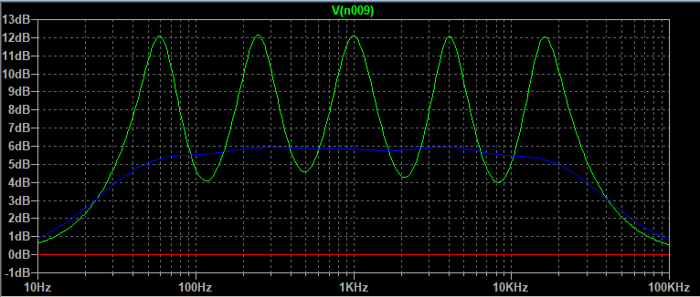

Figure 7 Spice Simulation of the Upper and Lower Halves of the Slider Pots.
For a verbal description click here.
Upon seeing this I said to myself "This isn't right. I can't show this. They'll laugh me off the web." My next step was to get out the actual equalizer. I found it didn't work so I did what you would expect. I found a piece of melted solder wedged in under a vertical mount capacitor that was shorting out the signal. "How did that affect both channels." I wondered. While I was at it I repaired the LED power indicator light which had not worked for many years. Back together and setup for testing.

Figure 8 Photograph showing the equalizer, Analog Discovery, and Computer.
The figure caption is all the verbal description that is needed.
You can sort of see it on the computer screen but here is a proper view of the four settings used in the Spice simulations shown above.


Figure 9 Four part picture showing +12, +6, -6, and -12 dB settings on the real equalizer..
The correspondence between the simulation and the real item is nothing less than astounding.
That's all the verbal description you need.
Just in case you are curious, the fifth graph shows the phase angle for all controls at -12 dB.
If you look back at the schematic above you will see that the value of the series resistor is quite different for different frequency bands. Ideally the value of this resistor would be the same in every band. The total resistance in each tuned circuit is made up of the discrete resistor plus the resistance of the inductor. In the Spice simulation the inductor is ideal so the resistor is the only resistance in the circuit. The value of all 5 resistors is 330 ohms. I found this value by setting it for 12 dB of boost and cut at the peaks of the curves for pots all the way up or down. The close similarity between the simulated curves and the actual device is remarkable.
I think duplication of this circuit would not be practical. First, center tapped slide pots are somewhat rare. Second even if you can get them they will most likely be linear. The pots used by Heath have a pronounced nonlinear taper. The resistance from either end to center is 25 k ohms. If the wiper is set half way between the center tap and either end the resistance from the wiper to the end is 1.1 k ohms. That's a shame because the circuit could easily be adapted to tubes and work rather well. Since I no longer have a use for the Heathkit eq I might just gut it except for the controls and rebuild it with tubes. Don't hold me to that.

Figure 10 Showing no Difference From Figure 7.
Going back to the simulation used to make figure 7 I removed the ground from only one band, the one in the middle. If it did make any difference it would be immediately obvious in figure 10. Adding the ground does make the circuit easier to understand but that appears to be its only benefit.
It Still Works Without the Ground, It's Just A Lot Harder To Explain.
Below you will find the equivalent circuit of equalizer with all pots combined in parallel.

Figure 11 Equivalent Circuit With Ground Removed and Pot Centered.
For a verbal description click here.
This is not going to be easy because all intuition fails us. I have gone so far as to modify my pot symbol to show the wiper in the exact center. Let's start assuming nothing connected to the wiper. That would be the case if we injected DC into an equalizer circuit because the capacitors in the series tuned circuits would prevent the passage of direct current. If we apply 1 VDC to the terminal on the left, the amplifier will pass the voltage with unity gain. To remind you of the first law of op amps, both inputs will always be at the same potential. That means that both ends of the pot will be at the same potential. There isn't any current in the wipers because of the capacitors. If there is no voltage across a resistor there is no current flowing in it by the law of Mister Ohm. Current does not flow into or out of the inputs of the op amp because it is an F E T input amp. This forces us to the conclusion that there is no current in either Ri or Rf. Consequently the output of OA1, both inputs of OA2, and the output of OA2 are at the same potential, namely 1 volt DC.
But What About AC?
Now we'll apply an alternating test voltage to the input at the left. Whatever the test frequency it's going to be close enough to one of the tuned circuit resonances for current to flow through it. That's going to pull the center of the pot closer to ground. Current will now flow through the pot. By the first law of op amps the two ends of the pot must be at the same voltage. The only way for the center of the pot to be at a voltage different from the ends while the ends are at the same voltage is for current to flow in (or out) of both ends of the pot. This requires that the currents in Ri and Rf must be equal and in opposite directions.Now the second law of op amps comes into play. It states that "the output of the op amp will assume the voltage needed to prevent the first law from being violated." Let's take a snapshot of voltages and currents when the input wave is positive. The output of OA1 is positive and current is flowing from it and to the right through Ri. Then through the left hand half of the pot and to ground through one or more of the tuned circuits. Meanwhile current is flowing out of OA2 to the left through Rf. Then through the right hand half of the pot through one or more of the tuned circuits to ground.
Because the two halves of the pot have the same resistance the voltage across them will be equal. This satisfies the first law of op amps. This also says that the currents in each half of the pot are equal. Because Rf and Ri, have the same resistance values the voltage drop across them will be equal. Therefore the output voltages of OA1 and OA2 are equal. QED. With all pots set to center (flat) the gain of the system is unity for all audio frequencies.
Now for the case of one or more pots set to the left as shown in figure 12 below.

Figure 12 Equivalent With Pot Set to Cut Side.
For a verbal description click here.
The impedance of a series resonant circuit is minimum and usually quite low at resonance. Moving this low impedance from the center to the left end of the pot will cause an increase in current through Ri. The first and second laws of op amps work together to make both ends of the pot have the same voltage. There is more resistance from the right end of the pot to the wiper than there is from the left end to the wiper. It takes less current from the right than it does from the left to equalize the voltages at the ends of the pot. There will be less current through Rf, than through Ri. The output voltage of OA2 will be reduced to satisfy the second and first laws and the amplitude will be reduced at and near the resonant frequency of the tuned circuit. Thus moving the pot wiper to the left causes a cut in amplitude at and near the resonant frequency.
In figure 13 the pot has been moved to the right.

Figure 13 Equivalent Circuit With Pot Set to Boost Side.
For a verbal description click here.
Now the situation is reversed. More resistance from the left end to the wiper means less current through that part. This also means less current through Ri than through Rf. More current through Rf means a greater voltage drop and more output from OA2. Moving the pot wiper to the right causes the amplitude to be boosted at and near the resonant frequency. The output voltage from OA1 remains constant for the discussion of both figures 12 and 13.
A More Modern Circuit.
Below is a simplified version of the BSR EQ-110X equalizer. What are all those op amps doing there? They are obeying the laws of op amps.
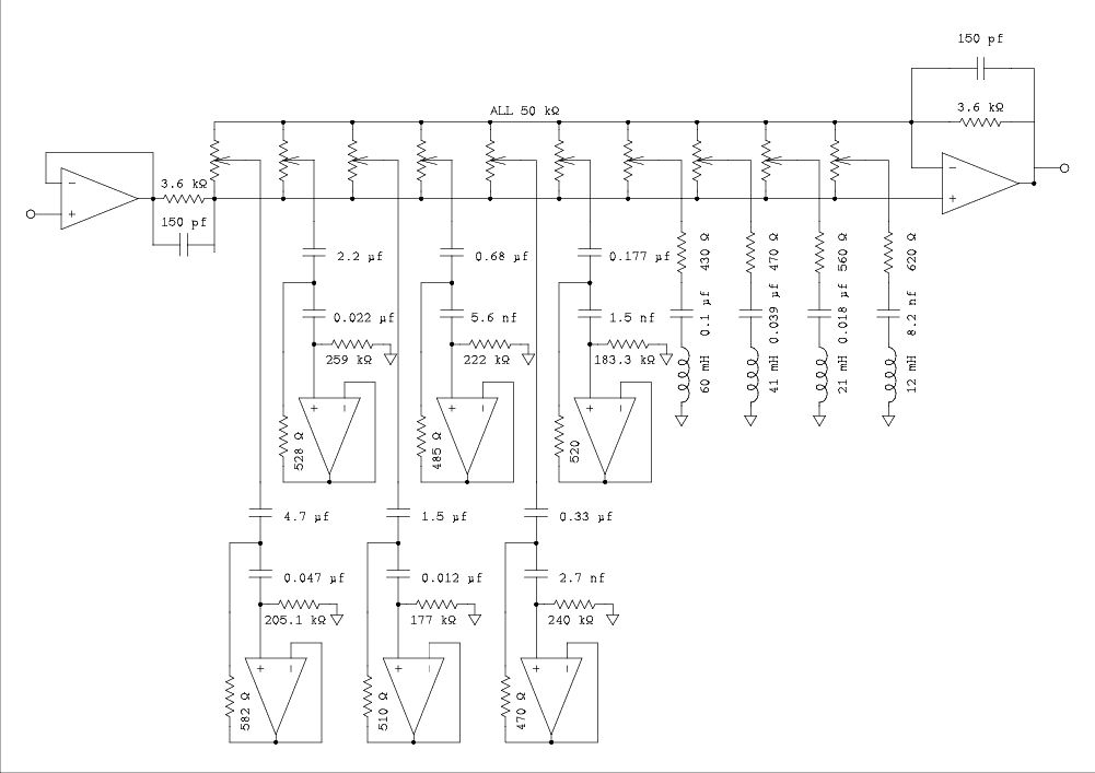
Figure 14 Simplified Schematic of BSR EQ-110X.
For a verbal description click here.
Look at the top four bands in figure 14 and compare to figure 4. Except for component values they are identical. These bands use inductors that appear similar to transistor radio IF transformers complete with adjustment slug. The bottom 6 bands use gyrators to replace real inductors. A real inductor for the 31 Hz band would have to be 5.6 Henrys. Apparently the performance of gyrators at frequencies of 1 kHz and lower is close enough to that of real inductors to make using them feasible. No doubt a high performance equalizer could be made with real inductors for all bands but its price would place it firmly in the professional audio market.
Here is the circuit of a gyrator and its resonating capacitor C2.

Figure 15 Circuit of a gyrator and its resonating capacitor C2.
For a verbal description click here.
The gyrator consists of C1, R1, R2, and the amplifier. C2 is the capacitor which tunes the inductance of the gyrator to a specific frequency.
Here Is How It Works.
The capacitor that is closest to the pot wiper is what tunes the circuit to resonance at the center frequency of the band in question. The next capacitor in line combines with the resistor to ground to form a phase lead network. This phase leading signal is fed to the noninverting input of the op amp which has been strapped for unity gain. This phase leading signal comes back to the junction of the two capacitors through a relatively low value resistor. The current that is fed back to the node is phase leading. In an inductor the current leads the applied voltage and thus the node where the two capacitors and resistor connect looks like one end of an inductor which has the other end grounded. The frequency of resonance is given byf0 = 1 / (2π*sqrt(R1R2C1C2))
Q = sqrt(R1R2C1C2) / (R2(C1 + C2))
The only equation that is missing is one that gives the inductance value. It can be obtained from the resonant frequency equation by removing C2 by division as follows.
First let's put the equation in terms of ω so we won't have to lug 2π around. Multiplying the f0 equation through by 2π gives,
ω = 1 / (sqrt(R1R2C1C2)).
Squaring gives,
ω2 = 1 / (R1R2C1C2).
Multiplying through by C2 gives,
ω2C2 = 1 / (R1R2C1).
We can now write,
ω ω C2 = 1 / (R1R2C1).
But,
ωC2 = 1 / Xc2.
Making the substitution,
ω / Xc2 = 1 / (R1R2C1).
Inverting both sides gives,
Xc2 / ω = (R1R2C1).
These calculations are being done at the resonant frequency, therefore,
XL = XC. Therefore,
XLG / ω = (R1R2C1).
Where XLG is the inductance of the gyrator.
But,
XLG = ωLG, or, LG = XLG / ω
Therefore the inductance of the gyrator is,
LG = (R1R2C1).
Derivation not shown but equation included for completeness,
RG ≈ R2.
Where RG is the resistive component of the inductance of the gyrator.
Although a special center tapped pot is not necessary for a graphic equalizer, it is clear from the simulations that a special taper is required. I haven't checked in detail but it may be that an audio taper is needed. The only catch is that it needs to taper on each end. That is, as the wiper is moved in from the end, either end the resistance changes slowly at first and more rapidly as the center point is approached. It is clear that the BSR unit does not have these special taper pots installed.
Conclusions On Graphic Equalizers.
The graphic equalizer is a powerful tool for modifying the sound of a recording. Whether you are a record producer, a live sound producer, or a listener, a graphic equalizer can often correct small mistakes in microphone placement, reduce a tendency for feedback, or knock down an unpleasant peak caused by room resonance.It seems a bit pointless to try to build one with tubes except for the reason "just to see if it can be done". The tube amplifier we will design in the next section can be used in a graphic equalizer as well as the parametric circuit for which it was developed. Those of us who build things around tubes don't need a reason. We do it just because it's fun.
The Parametric Equalizer.
The parametric EQ is different from the graphic because it only operates on one band of frequencies. The frequency is adjustable over most of the audio band. It has one control which is similar to the boost and cut controls on a graphic EQ. Many mixers have a parametric EQ in each channel. Because it only has two controls it doesn't take up a lot of panel space. It is superior to a graphic EQ for such applications as knocking down a feedback, or room resonance, peak because the frequency can be adjusted to hit the frequency of the peak right on instead of getting close.The Starting Point.
This project started when someone sent me a circuit of a commercial unit that contained a two channel graphic EQ and a parametric, one in each channel. This, no doubt, was a high end consumer grade device. He wanted to build it with tubes. I didn't have time to do any breadboarding but sent him a spice simulation that I hoped would work. Unfortunately it didn't. That's been a while and I no longer remember who it was nor do I have the original email message. So here you are sir, this one should work.Details Of The Wien Bridge.
Before we begin to analyze the circuit we need to know exactly what is a Wien bridge and how it works.The Wien bridge was originally developed and patented by Bill Hewlet for use in his low distortion audio oscillator. The diagram below actually shows only two sides of the bridge. The other two sides are a tungsten lamp and a resistor. However, it has become common usage to show this much of the circuit and still call it a bridge. Since the patent ran out the circuit has found many other uses than in an oscillator. This parametric equalizer is one of them.

Figure 16 Frequency Plot and Schematic of Basic Wien Bridge.
For a verbal description click here.
The Wien bridge has a curve almost identical to a low Q parallel tuned circuit connected in the plate circuit of a pentode tube. The resonant peak is shown in the center. Far from resonance there is a roll off of 20 dB per decade. It's resonant frequency can be brought down to single digit Hertz with reasonable values of R and C.
The resonant frequency is given by,
f = 1/(2π sqrt(R1 R2 C1 C2))
The attenuation at resonance is 1/3, if and only if R1 = R2, and C1 = C2.
If C1 is greater than C2 and, or, R2 is greater than R1 then attenuation is greater than 1/3.
If C2 is greater than C1 and, or, R1 is greater than R2 then attenuation is less than 1/3.
The Wien bridge is a very useful circuit in analog audio electronics.
The Wien Bridge In a Parametric Equalizer.
Here is the original circuit which is built around, guess what, an operational amplifier IC.

Figure 17 Schematic of IC based Parametric Equalizer.
For a verbal description click here.
The circuit that is connected from the wiper of the presents pot to the noninverting input of the op amp is the Wien bridge which we met in the previous section. The large coupling capacitor, 100 μF has no effect on the Wien bridge but the 680 k ohm resistors do. My guess is that the op amp IC used by the designers of the product is a BJT input device rather than an F E T. The bias current flowing through the frequency control rheostat to or from ground probably caused a change in the offset as the frequency was changed. So it was isolated from the op amp by a large capacitor. Then the 680 k ohm resistor was required to provide a return for the noninverting input. This would have altered the attenuation of the bridge at low frequencies when the frequency control is at high resistance. Another 680 k ohm resistor has been connected across the upper resistor in the bridge to make the attenuation constant for all settings of the frequency control. These parts can be omitted in a vacuum tube version of the equalizer.
The op amp is connected as an inverting amplifier so the input and output signals are always 180 degrees out of phase. If output and input have equal amplitude then the center of the pot will be at zero potential. This is insured by the fact the two resistors that set the gain are both 10 k ohms.
Say the presents pot is moved off center to the right. This will apply a signal to the Wien bridge which is out of phase with the input signal. For frequencies at and near the center frequency of the bridge a signal which is out of phase from the input will be applied to the noninverting input. The input signal is applied to the inverting input. When signals that are out of phase are applied one to the inverting input and the other to the noninverting input they are added together. This causes the circuit to have more gain at the center frequency than it does elsewhere in the audio spectrum. The Wien bridge does attenuate the signal somewhat. If it did not the circuit would be an oscillator. As it is the gain is increased by about 12 dB.
Now let's turn the presents pot to the left so the wiper is closer to the input end. Frequencies that are passed by the Wien bridge are in phase with the input so the inverting input and noninverting input get signals that are in phase. This causes the signals to subtract taking amplitude away from the input signal. Frequencies at and near the center frequency of the Wien bridge are reduced in amplitude by this subtraction while the rest of the spectrum is not changed in amplitude. The presents pot works exactly the same as one of the sliders in a graphic equalizer.
This is the simplest circuit around. There are others that use more op amps and have three controls, Frequency, Bandwidth, and presents. Since we are going to build it with tubes I think that one amplifier is all we can afford.
The Amplifier Designed with a little help from Circuit Simulation.
LT spice won't give you circuits out of the blue. You have to have some idea of what you want to do and I did.
- Even though it would be AC coupled it had to behave like an op amp so a differential input was a must.
- It had to have as much gain as possible with the minimum of tubes.
- Not only did it need high gain but bandwidth that would cover the audio band with a little to spare on each end.
- It had to be stable with feedback down to unity gain and even below.
- It must have a relatively low output impedance.
To satisfy number 1 a long tail pair with a current source in the cathodes seemed to be a natural. Especially since I have had plenty of experience with that particular configuration. A 12AX7 seemed to be the first choice because high gain was needed here.
To satisfy 2 and 3 a cascode amplifier came to mind. It can have more gain than a pentode without the division noise and with very little miller effect. In a cascode transconductance is where it's at and of all the 12A_7 tubes a 12AV7 has the highest.
The fewer stages an amplifier block has the easier it is to compensate on the high end. On the low end compensation gets easier if the number of RC coupling networks is kept to a minimum. I decided to try direct coupling from the long tail pair to the cascode amplifier.
Number 5 is easy, a cathode follower. Because the top plate of a cascode amplifier is at a higher voltage than the heater to cathode breakdown of most tubes, an RC coupler would have to be inserted here. For the follower I decided to round up the usual suspect and use a 12AU7. If only one channel is to be constructed The other triode can be used as a cathode follower at the input of the circuit. If you are planning to build two channels I suggest that the two triodes in one of the 12AU7s be used as the input cathode follower and the two in the other 12AU7 be used as the output stage of the amplifiers.
Developing the Amplifier.
I developed an amplifier, shown below, using LTspice that worked beautifully in simulation, (Note: This diagram does not give the final values used in the parametric section. Do not refer to this schematic when building.)
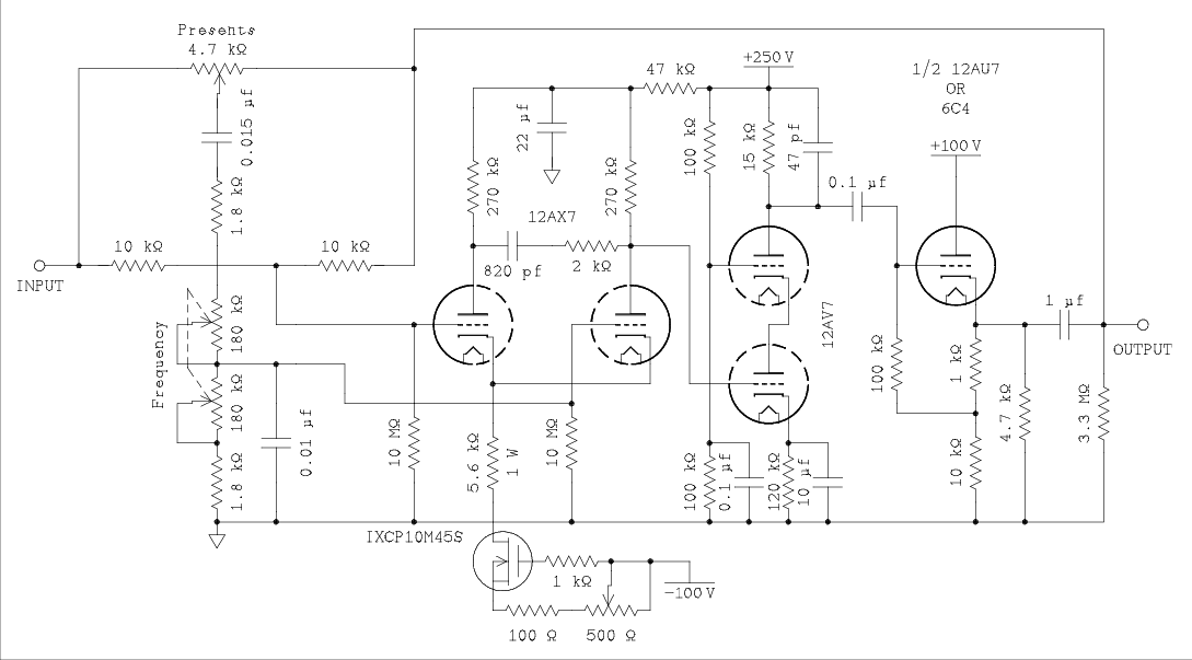
Figure 18 Initial Version of Tube Amplifier for Parametric EQ.
For a verbal description click here.
but when I built it and closed up the feedback loop it was a 100 kHz oscillator. I spent the next two months running frequency responses on the Analog Discovery and trying to get a decent Bode response on both the high and low ends
So after two months of real time and many unlogged hours at the bench the schematic of the amplifier that worked is shown in figure 21. But I'm getting ahead of myself.
Frequency response with the Analog Discovery Pro.
When setting up the analog discovery for some really serious work I found that when its signal generator is set to 10 millivolts and below there is a great deal of noise on it. In fact there was almost as much noise as signal. Surprisingly the signal didn't come out of the amplifier looking like that. The only thing I can conclude is that most of the noise is above the passband of the amplifier. However, the noisy signal is fed to channel 1 of the scope for phase readings. I don't think that readings could be very accurate with all of this noise. My solution is shown in figure 19 below.

Figure 19 Amplifier Test Setup.
For a verbal description click here.
The signal generator is set to 1 volt which is fed to channel 1 of the scope. After the 40 dB attenuator the signal is 10 millivolts which is what the amplifier needs. The only problem is that the gain of the amplifier comes out 40 dB lower than it actually is. I couldn't find a way to add an offset to the dB scale. I think this would be a very good addition to the software. Are you listening Digilant? You will note that although the simulation says the amplifier is stable at unity gain the measurements on the real amplifier make it clear that it is not. The gain is well above unity at zero phase on the high end.

Figure 20 Open Loop Gain and phase of Breadboarded Amplifier.
For a verbal description click here.
I'll spare you the details of the struggles of the last 16 days. I spent many hours running the low frequency response of the real amplifier using the Analog Discovery Pro. A scan from 1 Hz to 1 kHz takes 6 minutes and 9 seconds. From 100 millihertz to 1 kHz takes approximately 45 minutes. From 10 millihertz to 1 kHz takes approximately 5 hours. Sixteen periods of each input frequency are required to obtain the data for display.
I decided that I might not live long enough to compensate an AC coupled amplifier. The alternative is to make it more like an op amp with direct coupling throughout. That turned out to be easier than I had thought. Here is the schematic at the current state of development.

Figure 21, DC Coupled Amplifier, Closer to True Op Amp.
For a verbal description click here
You may be wondering why there is a 10 k ohm resistor on the left side of the diagram which is connected between the output and ground. Well, I'll tell you why. In the next diagram this will become the feedback resistor which will be connected from output to inverting input. The inverting input is a virtual ground so the feedback resistor is a load on the amplifier. I want to get you accustomed to thinking of the feedback network as a load on the amplifier the same as any other resistances or impedances that may be connected there.
The network consisting of the 330 kΩ resistor, 150 kΩ resistor, and the 100 kΩ pot, is both a level shifter and an attenuator. The level shifting is wanted, the attenuation is not. This was, and still is, common practice in tube op amp circuits because there is no PNP tube. Too bad. In this case the attenuation side effect of the level shifter became useful for the insertion of a lead/lag compensating network. This actually simplified the high frequency compensation of the amplifier although there were several false starts in this area before I arrived at this solution.

Figure 22, Open Loop Gain of DC Coupled Amplifier.
For a verbal description click here
Remember to add 40 to the vertical scale of the top graph.
Above is the open loop response of the real amplifier taken with the Analog Discovery. The plot shows stability because the gain is already below unity at 1 MHz while the phase is about 25 degrees as it approaches zero. Also where the gain is unity, 0 dB, the phase is about 50 degrees. It is hoped that this is not enough to sustain oscillation.
The gain can be seen falling off below 10 Hz. Remember that zero on the scale is 40 dB of gain. The gain does not fall to zero, minus infinity dB, below 1 Hz as would be the case with a capacitor coupled amplifier. The fall off is due to the cathode bypass capacitor on the cascode amplifier.
You may be wondering why the 47 kΩ and 22 μF filter doesn't cause a low frequency roll off. The 47 kΩ carries the sum of the two 12AX7 plate currents. The sum of the cathode currents is regulated by a current sink. The current through the 47 kΩ never changes. Removing the capacitor would probably have no effect but it is left in place so the circuit will look normal.
Closing the loop.
Here are the results of testing the real amplifier in closed loop configuration. First the schematic.

Figure 23, Schematic of DC Coupled Amplifier with negative feedback.
For a verbal description click here.
I tested the amplifier set to gains of 20 dB, 10 dB, 0 dB, -10 dB, and -20 dB. Only the gain of 0 dB, unity gain, is shown here.

Figure 24,Gain and phase graph for 0 dB (unity gain).
For a verbal description click here.
Adding the parametric circuit to the tube amplifier.

Figure 25, Schematic of Complete Parametric Equalizer.
For a verbal description click here.
And here is the simulation of the circuit.

Figure 26, LTspice Simulation of the circuit of Figure 25.
For a verbal description click here.
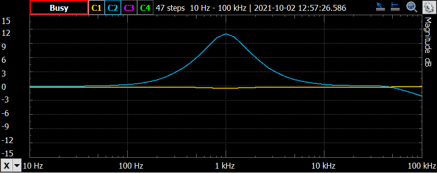

FIGURE 27, IT'S THE REAL THING.
For a verbal description click here.
One thing you might notice is that grid return resistors have been eliminated. Well, silicon op amps don't have return resistors on the inputs. The external circuit is supposed to provide that function. The two 10 k ohm resistors do the job for the inverting input. The 100 k ohm resistor is to make sure to discharge any coupling capacitors that may be connected there. The noninverting input always needs a return to circuit common. It is provided by the lower frequency pot in the Wien bridge circuit. The original silicon circuit had a DC blocking capacitor between the Wien bridge and the noninverting input. There was a 680 k ohm resistor to ground to keep the input where it belonged. There was another 680 k across the upper part of the bridge. I suspect that they were using a bipolar input op amp IC and the output level changed as the frequency control was turned. With tubes we have no such problem.
Having a breadboarded version of the equalizer meant I could plug it into my stereo and listen to it. This is not possible with an LTspice simulation. I have been listening to The Brothers Four's Greatest Hits. The effect the equalizer has on normal music is not something you would want to sit and listen to. But it is fun to play with.
A Power Supply.
If I omit this section I will get emails requesting a power supply circuit so why not provide one. Here it is.
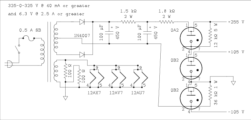
Figure 28, A Power Supply for the Amplifier.
For a verbal description click here.
The specifications for the transformer shouldn't be hard to match among the Hammond listings on Antique Electronics Supply. The values of the two resistors in parallel with the VR tubes are given for one amplifier. If you are planning to build for stereo the values of the two resistors in parallel with the two VR tubes should be cut in half and the wattage rating increased appropriately. I recommend building the power supply on a separate chassis from the equalizer circuit.
Adjustment.
Now you are ready to give it a listen.
- Plug everything in and turn on the power. All three VR tubes should glow pink or purple.
- Connect a DC voltmeter to the cathode of the bottom triode in the cascode amplifier.
- Adjust the pot in the source of the M O S F E T for a voltage of 78 volts.
- Connect the voltmeter to the output of the amplifier.
- Adjust the other pot in the amplifier for a reading of zero.
- Allow the amplifier to warm up for 10 or 15 minutes.
- Repeat steps 2 through 5.
Changing the Circuit For Different Applications.
Suppose you made a live recording and found when you got home that there was a peak or null at some obvious frequency. You could use this circuit to boost or cut that frequency. You can get a higher and more narrow peak by making the values of the two capacitors farther apart.Say you wanted to use it to knock down a bass peak in your speakers. You could modify the Wien bridge circuit to cover a range of 10 to 100 Hz. This can be done by increasing the value of the resistors in series with the two pots. The frequency can be lowered by increasing the values of the two capacitors while keeping them in the same ratio to one another. Making the bottom capacitor smaller or the upper one larger will increase the height of the peak but if you carry this too far you will wind up with an oscillator. You could also use the same modification to increase the low bass below the normal range of your speakers but you could run into the power limits of your amplifier or if you have a power house of an amplifier you could damage your speakers, so be careful.
The frequency pot.
The resonant frequency of a Wien bridge is given by,f = 1/(2*π*R*sqrt(C1*C2))
Where both resistors have the same value. R is the value of the resistors and C1 is the top capacitor while C2 is the bottom capacitor. The frequency is proportional to 1/R. The 500 k ohm variable resistor (pot) in figure 25 gives a frequency of 68.1 Hz when set to maximum. Decreasing the pot's resistance increases the frequency. If a linear pot were to be used the first decade would be covered as the pot decreased from 500 k ohms to 50 k ohms. Assuming 300 degrees of pot rotation this would take place in 270 degrees and the rest of the frequency range in 30 degrees. What is needed here is a dual reverse audio taper pot. Some early TV sets used reverse audio taper for the contrast control but finding a dual one is probably impossible. For my breadboard circuit I wired a conventional audio taper pot backward which meant that the highest frequency was fully counter clockwise. If I were going to build this for daily use I would get some of those plastic gears used by kids to build robots and gear the frequency pot for reverse action so clockwise rotation of the frequency control would increase the frequency.
Conclusion.
If you have a recording studio with even a moderately priced mixer it has a parametric equalizer in every channel. If you have a very small recording setup you might find one channel of this circuit to be useful. Your need for it is likely to be altering the timbre of one voice or instrument so only one channel should be needed.If you want it for your stereo entertainment system you should build two channels. If that's what you want I won't second guess you. For myself I find that playing with the controls for a few minutes to be amusing but it's not something I would install in my system and switch in every day. But as that comedian used to say "different strokes for different folks". What was his name?