Learning LT Spice.
Lesson 8

Click here to download a PDF of this page.

Table of Contents.

Lesson 1: Fundamental Drawing Skills and a Simple Simulation.
Lesson 2: Introduction to Frequency and transient Analysis.
Lesson 3: Configuring LT Spice and more Drawing controls.
Lesson 4: Locating, modifying, and installing vacuum tube models.
Lesson 5: Operating point of vacuum tube circuits. Introduction to stepping and plate curves.
Lesson 6: Finding, installing, and using, potentiometer symbols and models.
Lesson 7: Transient analysis of unregulated power supplies.
Lesson 8: Transient analysis of Regulated power supplies. This page.
Lesson 9: Transient and frequency analysis of amplifiers with feedback.
Lesson 10: Lossless transformers.
Lesson 11: Making symbols and models.

Lesson 8
Transient Analysis of Regulated Power Supplies.

H2>What you will learn in lesson Eight. How to:.

1. Explain the difference in performance between an adjustable power supply and a regulated adjustable power supply
2. Explain the difference in circuitry between an adjustable power supply and a regulated adjustable power supply
3. Use the load switch and transient analysis from lesson 7 To test an adjusting circuit to determine if it is regulated or not.
4. Use stepping to determine the proper value for a capacitor that is connected across the output terminals.
5. Use the load switch and transient analysis from lesson 7 To measure the output voltage of a simple regulator circuit at 1/3 load and full load.
6. Use zooming and scale changing to accurately measure the ripple at 1/3 load and full load.
7. Use stepping to determine the maximum and minimum voltages of a regulator circuit.

Static testing of power supplies.

This doesn't mean static you hear on the radio, it means standing still. The power supply is turned off, a resistive load is connected along with voltmeters and current meters to show what is going on. The supply is turned on and readings taken. The supply is turned off the load resistor is changed and when the supply is turned on again a new set of readings is taken. The main piece of information that comes out of static testing is the load regulation. The equation is,

%Reg = 100 * (VNL - VFL) / VNL.

Where VNL = no load voltage, and VFL = full load voltage. Full load current is one of the main design parameters and is determined by the designer.

It is usual for an oscilloscope to be connected to measure ripple but instantaneous response to changing loads is not part of static analysis.

An adjustable power supply is not necessarily regulated.

If you walk into a student electronics lab and see a power supply with a knob labeled voltage adjust, it may or may not be regulated. The most basic version of an adjustable but not regulated power supply is shown in Figure 8.1.

Figure 8.1 Simple adjustable power supply.

The item between the two switches is a variable transformer more commonly known as a Variac®. (Note: Registered trademarks should not be used in formal writing unless it is unavoidable.) The voltage output of a variable transformer is only very slightly effected by load current. The transformer, rectifier, and filter, each make their contribution to load voltage reduction and it all adds up.

Implementing figure 8.1 with real components would need a few changes from the schematic. First of all 500 volt capacitors are a little hard to find and I have never seen 100 μF 500 volt caps. So two lower voltage capacitors would have to be connected in series. The could be 250 volts but that would leave no margin for error. 350 volts would be preferable . 450 volts would not be better so why spend the extra money. As for me I have lots of 450 volt capacitors in stock so I tend to use them rather than making up a special order for each project. Also 1N4007s are marginal for the job. There are 1200 volt rectifiers but I don't have the number in hand at the moment. If you actually did build this circuit I would highly recommend their use.

This power supply is adjustable and well filtered against ripple from the AC line but it is not regulated. As you will shortly see.

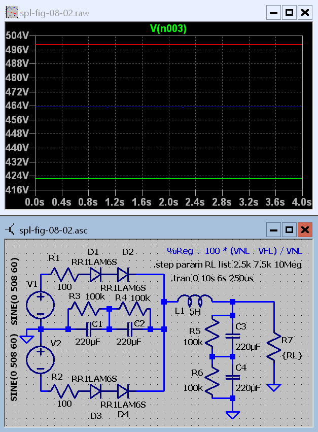
Figure 8.2 Static testing of the simple power supply.

Have you ever wondered what professors talk about in faculty meetings?

So, I am trying to figure out just how much to give the students and how much I should ask them to do for themselves. If I give them everything they won't learn anything. If I don't give them anything, that is I ask them to draw all the schematics themselves, they won't do it and will still learn nothing. Obviously what I need to do is fall somewhere between these two extremes. The question is exactly where between. I know from my many years of teaching in person classes that every student is different. Some will need to have quite a lot given. Others won't need or even want to have a lot given to them, they would rather do it themselves. Once again I am in a situation of on one hand this and on the other hand that. So, I will give them some schematic files and ask them to add a little to them to make the complete working schematic.

Meeting adjourned.

So, I will start you on your way to figure 8.2 by downloading this file.
Save the file in the same folder where you have put all other learning LTspice schematic files. Start LTspice and open the file you just downloaded. As soon as it is in and before doing a single thing else select Save as and save it under the name "spl-fig-08-02". Spice will assign the proper file name extension.

Now look at what is on the spice drawing board. You should have a circuit that has two sine wave generators, 4 resistors, 4 diodes, and 2 capacitors. Compare it with the schematic portion of Figure 8.2. Your mission, should you decide to accept it, is to fill in the missing parts. Add L1, C3, R5, C4, R6, and R7. You also need to type the three lines of text. The one in blue is a comment. When you press the letter S to put text on the schematic a box will come up that has a place to type text but above it are two radio buttons, one for "Comment" and the other for "Spice directive". The two lines that are in black are spice directives that are required to make the simulation work. Don't forget the leading period on the directives.

The two capacitors that are in series , each one with a resistor in parallel with it are the duplicate of the one that is between the two diodes. If you want to get fancy you can use ctrl C to copy the capacitors and resistors. After you press ctrl C and draw the box you can move the components outside the other parts and press ctrl R to rotate it. Move it to where you want it and left click. "Now he tells me."

Even though we are using transient analysis to get the output this is still a static test. We have waited long enough for starting transients to die down. As suggested below, once you have it in your own computer you can change the parameters in the .tran directive and see what you want to on whatever time scale you want.

Simulating figure 8.1 in spice has its pitfalls as well. Although capacitors have no voltage limit in LTspice I have shown seriesed capacitors so I could also show the equalizing resistors. They constitute a minimum load current on the supply which can effect it's no load voltage. In spice, Silicon diodes are modeled with their reverse breakdown voltage. LTspice doesn't appear to come with any diodes with reverse voltages any higher than 600 volts so I had to series two diodes on each side to make the power supply work properly.

It would be possible to model a transformer and power it from a single voltage source but transformers are hard to model and most spice users, myself included, don't really know how to make a realistic transformer in spice. So the center tapped transformer secondary is replaced by a pair of voltage sources in series. These generators have zero output resistance while a real transformer has an amount of winding resistance which can easily be measured with common hobby test equipment. Therefore, the two 100 ohm resistors in series with the diodes.

Before I put in the resistors the supply had a regulation figure of 3.5 %. This figure is totally outside the realm of reality. With the resistors installed it has a more real regulation figure of 15.4 %. In the formula given as a comment VNL is the no load voltage and VFL is the full load voltage. Throughout this page I will be taking full load current as 200 mA.

If you have duplicated this circuit in your own copy of LTspice there is something interesting to be seen. Right click on the ".tran" directive and change "time to start taking data to 0 (zero). Them run it. The damped oscillation is caused by an LC resonant circuit that was excited by the turn on transient. Change the stop time to about half a second or less to stretch out the cycles. Use the cursor to get an accurate measurement of the period of oscillation and see if you can figure out which L and C are causing the ringing. This is a common phenomenon in power supplies of this kind. It is not noticed because it does no damage and usually does not produce any observable effect.

Is this next one a regulated power supply?

Figure 8.3 More complex adjustable power supply.

I know but I'm not telling. Yet. Let's draw it up and simulate it.

What I'm going to do next is dangerous. The danger is loss of a file. If you are restarting work after a break you will have to start LTspice and reopen the file "spl-fig-08-02. If you are continuing work you already have it loaded. Before doing anything else select "Save as" from the files menu and save the file under the name "spl-fig-08-04". If you put it off saying to yourself "I'll save it under a different name later". Do that and you are setting yourself up for a lost file as it is written over by a completely different file but with the same name. OK, do you have it saved under the new name? Promise?

Now. You want to keep everything to the left of L1 and delete L1 and everything to its right. You can press F5 and delete items one at a time but this gets tedious because every little connecting wire must be deleted. Use the scissors to draw a box around everything to the right of L1. (Hold the left mouse button while moving the mouse. You will see the outline of the box.) Sometimes it can get a little tricky to distinguish between two objects that are close together. Start at the upper left corner above L1 and below the line of text allowing the left side of the box to cut across L1. Move down and to the right. Include everything else to the right except the lines of text. When you release the mouse button everything that was inside the box will disappear. Move the scissors over L1 and click. It will also be gone. Delete the short line that connected L1 to the vertical line. And finally, move the three lines of text to the left and up a little so they will be positioned above the rectifier part of the circuit as shown in figure 8.4.

You have two options.
1. Now draw in the four tetrode* tube symbols, the linear pot, the three resistors, and the two capacitors.
2. If you would rather have some help with that click to download file.
Place this file in the same folder where you have been saving learning LTspice schematic files.
Load the file into spice, press ctrl C, draw a box to copy, and ctrl tab to switch to the power supply.
Position the tubes as shown in figure 8.4 and click to lock them in place.
Ctrl tab back to the tubes and close it by pressing ctrl F4.
If asked if you want to save the file say no.
First you will connect the plates and screen grids of the 6L6GCs to the diode cathodes.

* When I was learning electronics the 6L6 tube was known as a beam tetrode. Now they are often called power pentodes. The suppressor grid which is shown in tube data sheets is often connected to the cathode. LTspice takes a shortcut by omitting the suppressor grid from the symbol and connecting it to the cathode in the model. Therefore the symbol is a tetrode not a pentode.

Finish the diagram by drawing in U5 - the 500 k pot, R9 - 100 k resistor, C3 - 22 μF capacitor, C4 - 47 μF capacitor, and ground symbols.
Don't forget to change the value of the pot from "R=10k" to "R=500k".
Also change the pot setting from "w=0.5" to "w=1".
W=0 is fully counter clockwise, w=1 is fully clockwise, and w=0.5 is half way between.
Make sure that the ".step" and ".tran" directives are in black text. If they are not do this.
Right click on the line of text. In the box that comes up click the radio button next to directive.
Then click OK.
If any of the values are different from the diagram, right click the text to edit them.

Figure 8.4 Static Regulation analysis of more complicated power supply.

In the graphs that accompany figures 8.2 and 8.4 the green line is VFL and the red line VNL. Calculate the %Reg (percent regulation) for both figures. Note that in 8.4 some ripple is visible in the full load line while none is visible in figure 8.2. I think you have already figured it out. 8.4 is not a regulated power supply although it uses some of the parts of a voltage regulator.

Dynamic regulation test.

First let's convert figure 8.4 into figure 8.5. If it's not already in, load figure 8.4.
Select save as from the files menu. Save the diagram as "spl-fig-08-05.
Delete R10 and its associated wiring.
Move C4 and the output label over to the right of the diagram as shown in figure 8.5.
Delete any stray blue lines and ground symbols left behind by the removal of R10 and moving C4.
Download the Dynamic test load.
This is figure spl-fig-08-80. Save it in the folder with the other spice lessons files.
Switch back to LTspice and open spl-fig-08-80----.asc you just downloaded.
Press ctrl C to copy, select the entire diagram, ctrl tab to spl-fig-08-05, and place it in figure 8.5 as shown in figure 8.5.
Ctrl tab back to spl-fig-08-80 and close it with ctrl F4. If you are asked to save it click no. Connect the upper input line of the dynamic test load to the cathodes of the 6L6GCs.
Connect the lower input line of the dynamic test load to any ground symbol.
In the three lines of text at the upper left of figure 8.5 change the ones that are in black to comments by turning them blue.

Here is how to do that. Right click on the black text.
When the box comes up press the esc key.
In the box which takes its place click the Comment radio button.
Click OK.

In the 6 lines of text just above S1 change the two lines that are in blue but spice directives to black.
Right click on the text and the box that comes up will have two radio buttons. One for Comment and one for SPICE Directive. Click on the latter.
Now run the simulation.

Figure 8.5 Dynamic Regulation analysis of more complicated power supply.

This was practice for when power supplies get more complicated. If you were planning to build something similar to this power supply you could use this simulation to optimize its performance. For example, the very long recovery time is caused by the long time constant of the 500 k ohm pot in parallel with the 100 k ohm resistor and the 22 μF capacitor. The obvious thing to do is make the capacitor smaller. But a point will be reached where the ripple in the output starts to increase. A compromise will likely have to be made between recovery time and ripple. A power supply of this kind is likely to be used where adjustability is required but tight voltage regulation is not needed.

True regulated power supplies.

The block diagram of Figure 8.6 shows the essential elements of a regulated power supply.

Figure 8.6 Block diagram of a generalized linear control system..

The output voltage of the regulator is compared to a reference. Any departure of the output voltage from the voltage that the designers or operator has set is known as the error signal. The error signal is passed to an amplifier and the amplifier passes it on to the controller. Figure 8.7 shows a regulated power supply made with triodes.

Figure 8.7 Simplest possible regulated power supply.

In figure 8.7 the reference is the 0B2 voltage regulator tube. This particular type maintains a voltage of approximately 107 volts across its terminals as the current varies from 5 to 30 mA. This maintains the voltage at the cathode of the lower triode at 107 volts. The grid of the triode is fed from a fixed voltage divider which applies 1/3 of the output voltage to the grid of the tube. This tube serves as both the comparison device and the amplifier.

The output of the amplifier feeds the controller which is another triode tube. This is the pass tube. It is a common plate amplifier which is better known as a cathode follower. In normal operation the grid of the lower triode is 1 or 2 volts negative with respect to the cathode. The grid of the upper triode can range from several volts to a few tens of volts more negative than its cathode. The upper tube is a power tube which is likely to have a lower amplification factor than the lower triode. A lower amplification factor usually means more voltage between grid and cathode in normal operation.

If a load suddenly demands more current from the pass tube the voltage at the cathode of the pass tube will fall. The voltage at the grid of the error amplifier, the lower triode, will become more negative which causes the plate current to decrease. The voltage at the cathode of the error amplifier is held constant by the voltage regulator tube. The voltage across the 100 k ohm resistor will decrease and the cathode current of the upper triode will increase to meet the demand for more current. The output voltage will change by a small amount but much less than we have seen with unregulated power supplies.

When simulating a vacuum tube circuit a model for the glow discharge voltage regulator tube is hard to find. The most logical substitute is a zener diode. But high voltage zeners have a large positive temperature coefficient which can cause the voltage to change by 5 volts or more as the zener warms up. Also, when simulating some power supply circuits I ran into a problem with unwanted feedback being passed from the rectifier/filter circuit to the cathode of the amplifier through a zener that had poor regulation. Your best bet for a substitute for the voltage regulator tube is a DC voltage source as shown in figure 8.8.1. (Note: I could have overcome the unwanted feedback problem by using a current source in the cathode of the zener. I didn't want to make the circuit any more complicated than it already is. In real circuits the temperature coefficient can be compensated for.)

The Simulation.

You may already be thinking that I am cheating because I have used 6L6GCs instead of the triode shown in figure 8.7. I say in my defense that the 6L6 tubes are triode connected. The amplification factor, μ, of a triode connected 6L6 is 8. (μ = Gm Rp where Gm = transconductance and Rp = plate resistance). That puts it down there with most of those heavy duty triode pass tubes.

Two things are on the simulation diagram that are not on figure 8.7. They are C3 and C4. C3 was added to increase the loop gain for 120 Hz and above, which will reduce the ripple. The higher the loop gain the less ripple there is in the output. C4 is to keep the output impedance of the regulator low at medium and high audio frequencies. But as figure 8.8.2 shows they introduce a problem. The green trace is for a C4 value of 0.047 μF which is barely different from no capacitor at all. When the load current increases in a sudden step the voltage does really drop before being corrected as I described above. As it recovers it overshoots a little in the opposite direction before settling down to track the change in rectifier output but with considerably reduced amplitude. You don't have to take my word for it. Just add a trace for the voltage at the plate and screens of the 6L6s to the graph. I'll leave this one to you.

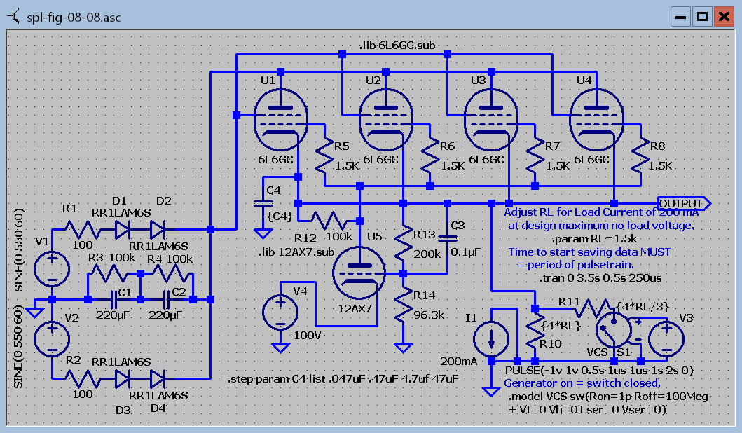
Figure 8.8.1 Simulation of Simplest possible regulated power supply.

The directive at the bottom center of the diagram tells spice to run the simulation for 4 different values of C4, namely 0.047, 0.47, 4.7, and 47 μF. The graph that results is shown in figure 8.8.2.

Note that the voltage source, V4, in the cathode of U5, is set to 100 volts. The off-standard value of R14 is an attempt to calibrate the relationship between the value of R13 and the output voltage. The idea is to make it so that 1 k ohm of resistance equals 1 volt of output. This was not exactly achieved but comes fairly close. See under the heading "Min and max output voltages of figure 8.8.1".

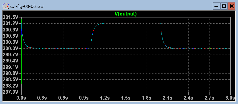
Figure 8.8.2 Four color graph showing response for four different values of C4.

Actually figure 8.8.2 shows traces for 4, that's four, different values of C4. The trace colors are as follows.
Green 0.047 μF,
Blue 0.47 μF,
Red 4.7 μF, and
Cyan 47 μF.
Do I hear someone asking what red trace? The red trace is hidden behind the cyan trace. This tells us that changing from 4.7 μF to 47 μF does not change the outcome enough to be significant. For subsequent simulations I set the value of C4 to 4.7 μF.

I wish there was some way I could show you a motion picture of the graph traces being drawn. You would see the higher capacitance traces covering parts of the lower capacitance ones. At the same time I am wishing, I am glad I can't, because if you really want to see the motion picture you will have to draw the schematic and run the simulation on your own computer.

Figure 8.8.3 gives the impression that getting the value of C4 right increased the peak to peak voltage of the square wave. But look again. Always look at the scale values before jumping to a conclusion. If you read the horizontal parts of the wave on the vertical scale of both graphs you will get the same values for the high and the low levels.

Figure 8.8.3.1 Simulation showing power supply with load that switches between 1/3 load and full load.

It is clear in the above figure that there is more ripple when the power supply is heavily loaded than when it is not so heavily loaded. But how much ripple is there? You don't have to change the time scale in the .tran directive and run the simulation again. The data is already there with 250 microsecond resolution. All you need to do is tell spice that you want to see it. . You can do that by first zooming in on a small part of the graph with the zoom to rectangle command.

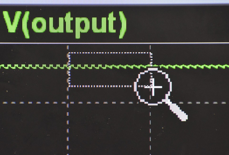
Figure 8.8.3.2 Shows how the zoom to rectangle is used to produce a detailed graph of part of the wave.

After you release the mouse button on the second corner of the rectangle you will see what you asked for. But it can use a little scale adjustment.

Figure 8.8.3.3 Shows the results from zooming to rectangle in figure 8.8.3.2.

I wanted 1.5 seconds to 1.6 seconds. As you can see I missed the right end of the intended expanse. But that's easy enough to fix. Just right click on the horizontal scale and change right limit from 1.61 to 1.60.

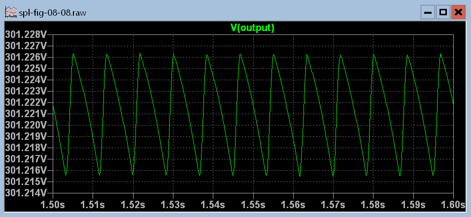
Figure 8.8.4 Shows how changing the vertical scale can permit accurate reading of the peak to peak ripple at 1/3 load.

The vertical scale needs a bit of fine tuning as well. Here's where it may seem impossible to make LTspice give you exactly what you want. Right click on the vertical scale and set the graph top, Tic, and Bottom. To what you want. You may or may not get what you asked for or what you expect. For example if you set the tick value to 2 millivolts a human would presume that you want the tick marks to fall on even numbers of millivolts. But if the Bottom value is set to an odd number of millivolts all the ticks will fall on odd numbers. LTspice doesn't have the smarts to figure that out and gives you exactly what you ask for instead of what you want. So right click again and set the top and bottom values to even numbers of millivolts.

Then suppose you set the Tick value to 1 mV. After clicking OK the vertical scale only has 3 values on it. One at the top, one in the middle, and one at the bottom. This is LTspice's signal that you have asked for more ticks than there is room for on the scale. If you are determined to get the number you want try clicking on and dragging the lower edge of the graph window downward until the scale appears how you want it. This usually happens before you run out of screen.

Figure 8.8.5 The same procedure of zooming and changing scales works for peak to peak ripple at full load.

For figure 8.8.5 the figure caption says all that needs to be said. Meanwhile we will convert figure 8.8.1 to an adjustable regulator and investigate its minimum and maximum voltages.

Min and max output voltages of figure 8.8.1.

Making this circuit an adjustable regulator is no big deal. All we have to do is replace R13 with a rheostat connected potentiometer. In the simulation it's even easier. All we need to do is to replace the value of R13 (300 k) with a variable name. How about {R13}. Now we can use a .step directive to step through several different values of R13 to see what happens to the output. It would be nice if we could make it so the regulator circuit would give us an output of 1 volt for every 1 k ohm of resistance in R13. The only problem is that the cathode of the amplifier is at 100 volts not zero volts. So the formula for R13 has to be,

R13 = (Vo - 100V) / 1 mA

I tried to trim the value of R14 to get right on this ideal equation but the simulation is a little off from it. Maybe connecting a small fixed resistor in series with R13 would work. The value of this resistor could be adjusted to make the equation hold. I'll leave that one for another day and a better regulator circuit.

We are going to change the nature of the load. Instead of a resistor we will use a constant current sink. That makes the amount of current being drawn independent of the voltage. When testing for maximum voltage the specified full load current is used. We wouldn't want to publish a specification of max volts with half load and have the users' find that it won't go that high when delivering the specified full load current.

Figure 8.8.6 Output voltage for 5 different values of R13 covering most of the range of adjustment.

.step param R13 50k 300k 50k

The directive tells spice to step R13 from 50 kΩ to 300 kΩ in steps of 50 kΩ.

The trace colors and corresponding resistor values are as follows.
Green, 50 kΩ.
Blue, 100 kΩ.
Red, 150 kΩ.
Cyan, 200 kΩ.
Magenta, 250 kΩ.
Gray, 300 kΩ.

The point where we start getting a lot of ripple is out of bounds for the maximum voltage specification. Therefore we will look at the maximum voltage region with higher resolution.

Figure 8.8.7.1 High resolution of output voltage showing upper limit.

.step param R13 240k 255k 5k

Trace resistor values are as follows.
Green, 240 kΩ.
Blue, 245 kΩ.
Red, 250 kΩ.
Cyan, 255 kΩ.

The cyan trace has the characteristics showing the effect of the ripple valley of the rectified and filtered voltage that is present at the diode cathodes. For a thorough discussion of ripple valley voltage see this link.

Figure 8.8.7.2 shows an idealized drawing of the ripple voltage and its effect if the ripple valley is too low for the regulator to sustain its voltage. The ideal voltage regulator would deliver the regulated output voltage even if the input voltage, voltage at the plates of the pass tubes, was equal to the output voltage. But if the wanted output voltage was greater than the input voltage it wouldn't happen. The regulator cannot produce a higher voltage than it is given. Although when I was teaching I found that some students were unable to wrap their minds around the next logical step. It is true for tubes and also transistors that there must be some voltage drop across them for them to do their thing. The output voltage of a regulator MUST always be less than the input. By how much depends on the type of device being used as the pass element. If the rectifier and filter has an output of 500 volts. And the minimum drop across the pass tubes is 110 volts then the maximum available output voltage is 390 volts. But wait, as they say on TV, there's more. What if the rectifier - filter has some ripple on it. Say 15 volts. (Note: The ripple waveform is always below the peak.) That means the ripple valley voltage will be 485 volts. In order for the output of the regulator to have a minimum of ripple on it the output must be 110 volts less than the ripple valley voltage. The maximum output voltage is 500v - 15v - 110v = 375v

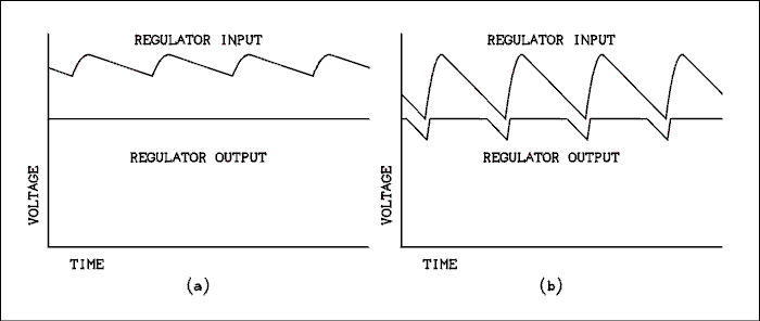
Figure 8.8.7.2 If the input voltage becomes too low the regulator will be unable to maintain output voltage.

Part (a) is good, part (b) is bad. Look back at figure 8.8.7.1. The cyan line shows a good resemblance to this drawn figure. All other traces are clean on the scale shown.

If I were writing up this power supply for a construction article, and I don't think I would, I might be talked into stating that it has a maximum voltage of 350 volts. Now let's check the minimum voltage. We do that with no load. A load would pull the voltage down and give it a better specification than would be seen with no load.

Figure 8.8.8 Minimum voltage test of simple regulator.

.step param R13 50k 100k 10k

That gives us a good idea of where the lower limit is. Now let's look for the limit with finer steps.

Figure 8.8.9 Minimum voltage test of simple regulator.

.step param R13 68k 82k 2k

From the red line it looks like this could be called a 174 to 350 volt power supply. However, I would rather call it a 175 to 350 volt power supply. I didn't say this was a good circuit, I just said it was a simple one. My original source was a 250 volt fixed voltage power supply that didn't even have a trimming pot to fine adjust the voltage.

The cathode of the 12AX7 amplifier is at 100 volts so we couldn't expect the output to go below that value but why is the minimum voltage so high? Checking the plate of the 12AX7 which is also the grids of the 6L6s I found that the amplifier was very nearly in saturation at about 103 volts. Where is the rest going? There can only be one answer to that and you already know it. The output voltage is the cathode voltage of the 6L6s. With the grids at 103 volts and the cathodes at 175 volts most of the voltage is going into getting those big triode connected bottles turned down to a very low plate current.

You might be thinking of hanging a load resistor on the output to cause a few mA to be drawn to see if it might just pull the output voltage down to under 150 volts. But what might that do to the upper limit. It's going to pull it down some and because it's a resistor as opposed to a current sink it could well bring it under 300 volts. Well, that's a good one to try on your own.

One possible solution to this problem is to pentode connect the 6L6s. This will cause them to have a much higher amplification factor and it won't take as much negative bias to drive the tubes almost to cutoff. That may also improve the ripple performance as well.

Conclusion.

I started out to do several different power supply circuits but I realized that it would be the same thing over and over. You've been through it once. Now if you want to see how your favorite power supply circuit performs you have the tools to do it. For more information on power supplies than you probably want to know, click here.

DON'T FORGET TO SAVE THE DRAWING. .

If you can honestly checkoff each item on the list under the heading "What you will learn in lesson 8", you can go on to lesson 9, assuming I have written it by then.

This page last updated Thursday, May 19, 2022.

Home.